Masters thesis on Majorana systems
The PhD builds on earlier work in quantum information and non-local correlations.
My PhD work focuses on time-reversal-symmetry-breaking superconductors: materials where the superconducting state does more than simply conduct without resistance. It also breaks an important symmetry of the underlying equations, opening a path to rich microscopic structure and experimentally observable signatures.
The core task is to build microscopic theories that are physically motivated enough to say something real about experiment, rather than remaining abstract formal exercises.
That means:
Working at that level made a separate problem impossible to ignore. Scientific thinking is often split across too many tools, too many formats, and too much friction between writing, calculation, and collaboration.
That is a large part of why my research life expanded into software and systems-building. QuantaLumin, TutorLumin, and LuminOS all came from the same pressure: to make serious intellectual work more coherent.
The background chapters establish the conventional superconducting baseline, then narrow toward the thesis mechanism: TRSB from internal winding in multicomponent superconductors, the BdG and topological language used to analyse microscopic representatives, and the low-energy phase dynamics of coupled superconducting phases.
This thesis now supports a clear final boundary. Experimentally, both LaNiC and LaNiGa show superconducting time-reversal-symmetry breaking. The materials-faithful programme developed here therefore asks whether the minimal microscopic TRSB mechanisms advanced in the thesis can recover that fact on shared Wannier bases rather than only in reduced toy models.
The answer is scientifically useful even where it is negative. On the dense Fermi-aligned Wannier bases, the present reduced closure set does not recover TRSB as the thermodynamic ground state. For LaNiC, the seeded mixed-parity branch collapses onto the singlet control. For LaNiGa, interorbital unitary and nonunitary TRSB branches remain as self-consistent solutions, but both lie above the singlet control in free energy. This is not a demonstration that the materials are experimentally singlet superconductors. It is a demonstration that the current minimal materials-faithful closures do not yet explain the observed TRSB.
That distinction also clarifies the status of the two microscopic pictures developed across the thesis. The nonunitary multiorbital triplet mechanism has now been tested in a minimal materials-faithful form, and on the present reduced basis it is not selected as the preferred state. The singlet frustration or loop-supercurrent mechanism is not yet falsified by the material calculation, because the chapter-15 comparison used a conventional singlet control rather than the full frustrated multicomponent winding closure on the imported Wannier basis. The unified-theory chapter therefore remains a conceptual synthesis of the two languages, while a direct material-faithful realization of that equivalence remains open.
That is an appropriate place for a PhD thesis to stop. The thesis has established a reusable BdG and qttree framework, a real QE to Wannier to materials-study pipeline, a set of topological and reduced-model consequence studies, and a falsifiable materials comparison that sharply narrows what still needs to be explained. The remaining work is a coherent postdoctoral programme: richer closure families on the imported bases, explicit frustrated singlet loop closures in the materials setting, broader low-energy orbital reductions, and tighter quantitative comparison to experiment. Those are no longer missing foundations. They are the next research programme.
This tree holds thesis-facing result chapters only: cleaned narrative text,
selected figures, and stable data artifacts. Shared reusable code lives in the
common qttree package, while broader exploratory or supporting computational
material is kept outside the thesis narrative.
This section is the thesis-facing result narrative. It is intentionally limited to three chapters. The computational notebooks and reusable implementations live in QuLab; this section keeps the argument, the selected evidence, and the conclusions.
Together these chapters cover the current qulab.research results as a thesis
story rather than as a research-log index.
This section keeps thesis-level technical material without interrupting the main argument. Appendices should be narrow, cited from the chapter that uses them, and limited to derivations, reference tables, or supplementary constructions needed by the defended thesis.
This thesis took shape over a long period of reading, modelling, coding, and revision. I am grateful to the supervisors, collaborators, colleagues, and friends who helped sharpen the argument, challenged the weaker ideas, and kept the work moving when it would have been easier to leave it unfinished.
I am grateful to the University of Kent, and to the School of Engineering, Mathematics and Physics in particular, for the institutional setting in which this work was carried out. I also owe thanks to the wider condensed-matter and superconductivity community whose papers, preprints, seminars, and conversations provided both the materials context and the conceptual pressure that pushed this thesis toward its final form.
Finally, I thank my family and those close to me for their patience throughout the long and uneven process of finishing this work.
The live adaptive-scan workflow for this result family is now maintained in the canonical Notebook bundle:
~/Projects/Research/Notebook/content/unconventional-superconductivity/frustration-mediated-loop-supercurrent
That Notebook bundle retains code_40_adaptive_phase_space_expansion.py, the
publishable and quick-run parameter presets, and the operational notes for
targeted hybrid-global checks. The PhD tree now keeps only thesis-facing
chapters, figures, and stable artifacts.
This directory is a thesis content tree; keep workflow notes here for maintainers/agents only.
To attach a missing PDF to an existing Papis entry (library papers), use:
1papis -l papers addto --doc-folder /home/henry/Resources/Papers/<papis_id> -f /path/to/file.pdf --file-name '{doc[ref]}.pdf'Replace <papis_id> with the entry folder id and /path/to/file.pdf with the downloaded file path.
Guidelines for automated agents (and humans) modifying manuscripts intended for the Physical Review family of journals, with Physical Review Letters (PRL)–specific rules called out explicitly.
Primary references:
styleguide-pr.pdf)journals.aps.org/prl/authors)This repository’s manuscript sources should follow the conventions below.
Maintain the standard Physical Review ordering unless the target journal requires otherwise:
PRL title capitalization
(Non-PRL Physical Review journals commonly use sentence case; keep the repository’s target-journal setting consistent.)
Use the journal’s standard hierarchy and format headings consistently.
PRL generally uses run-in headings, not freestanding headings:
Introduction—Text follows hereIf a further level is used:
Global fit: Text…Theorems/lemmas/proofs:
… as shown in Ref. [1].(a), (b), … and cited as Fig. 1(a).(1), (2), (3), ….obs, av).DWBA, bcc).cutoff, not cut-off; output, not out-put).nonradioactive), but use hyphens where closing creates ambiguity or awkward doubling, or when attaching to proper nouns (e.g., non-Fermi).0.2, not .2).APS journals strongly encourage sharing data/code/software that support results.
PRL placement and styling
Data availability—Text follows…PRL
Appendix—Text… (single appendix)Appendix A—Text… (multiple appendixes)Appendix: Survey of results—Text… (single appendix with subtitle)When changing manuscript sources:
Fig. 1(a), Table I, etc.).Introduction—…) (PRL rule).Guidelines for automated agents (and humans) modifying manuscripts intended for the Physical Review family of journals, with Physical Review Letters (PRL)–specific rules called out explicitly.
Primary references:
styleguide-pr.pdf)journals.aps.org/prl/authors)This repository’s manuscript sources should follow the conventions below.
Maintain the standard Physical Review ordering unless the target journal requires otherwise:
PRL title capitalization
(Non-PRL Physical Review journals commonly use sentence case; keep the repository’s target-journal setting consistent.)
Use the journal’s standard hierarchy and format headings consistently.
PRL generally uses run-in headings, not freestanding headings:
Introduction—Text follows hereIf a further level is used:
Global fit: Text…Theorems/lemmas/proofs:
… as shown in Ref. [1].(a), (b), … and cited as Fig. 1(a).(1), (2), (3), ….obs, av).DWBA, bcc).cutoff, not cut-off; output, not out-put).nonradioactive), but use hyphens where closing creates ambiguity or awkward doubling, or when attaching to proper nouns (e.g., non-Fermi).0.2, not .2).APS journals strongly encourage sharing data/code/software that support results.
PRL placement and styling
Data availability—Text follows…PRL
Appendix—Text… (single appendix)Appendix A—Text… (multiple appendixes)Appendix: Survey of results—Text… (single appendix with subtitle)When changing manuscript sources:
Fig. 1(a), Table I, etc.).Introduction—…) (PRL rule).main.tex.figures/self_consistent_convergence_example.pngfigures/wannier_band_validation.pnghenry/qulab/qulab/research/int/scripts/generate_figures.py.qulab.core.scmft.benchmarks.self_consistent.repaired_int_kanamori.repaired_int_seed_comparison_benchmark.henry/qulab/qulab/research/int/data/lanix2_wannier/LaNiGa2_full_soc_icarus/qe_bands_validation_aligned.json.LaNiC2_zhang2018_soc_icarus/wannier90_hr.datLaNiGa2_full_soc_icarus/wannier90_hr.datDelta_upup and Delta_downdown amplitudes.U'=U-2J_H and J_P=J_H is the intended Kanamori convention unless explicitly overridden.This chapter presents a general framework for building the most general quadratic Hamiltonian consistent with the physical structure of the problem. That structure includes lattice translations, boundaries, inhomogeneous geometries, and defects; optional particle-hole (Nambu) doubling; internal structure such as sublattices, orbitals, and intra-cell positions; spin; and whatever set of symmetry generators is imposed for the model under consideration.
The same formalism is intended to cover both single-order and multi-order settings, including spatial textures, flux- or current-like phases, and regimes in which different orders either compete or coexist. In that sense, the aim of the chapter is not only to write down particular Hamiltonians, but to establish a general construction that can be applied across the later microscopic models in the thesis.
We also explain how this microscopic framework connects to, and generalises, the more macroscopic symmetry-based approach associated with Ginzburg and Landau.
Geometric input for the microscopic construction: a finite sample region with boundary , embedded in the ambient space and spanned by primitive lattice directions , , and . In the formalism below, this geometric data is encoded by the lattice Hilbert space together with the boundary conditions and mask operator.
Minimal tight-binding picture of a conductor. A local orbital energy sits on each site, while a hopping amplitude connects neighbouring sites. The quadratic Hamiltonians developed in this chapter promote this local on-site plus inter-site structure to the full lattice Nambu internal spin tensor product.
We fix the tensor-product order
All operators are written to respect this order. When Nambu space is absent, the factor is simply omitted and the formulas are interpreted in the normal, non-doubled space.
Fix a finite lattice with shape and boundary-condition label . Let 𝕄 be a defect/mask operator acting on .
Start from the “pure translation” shift 𝕊 defined by its action on site kets :
where specifies how is interpreted at the boundary.
To model inhomogeneous geometry, impurities, vacancies, or any other spatial inhomogeneity, let 𝕄 be a fixed site mask: a diagonal operator in the site basis with eigenvalues , selecting the active lattice degrees of freedom.
This equation defines the slash notation “”: the shift only connects active sites. Equivalently, one may work directly in the restricted active-site subspace. The same masking can be written compactly as:
Embed the masked shift into the full Hilbert space using the fixed order:
Accordingly, any quadratic term may be written as a sum of objects of the form (shift on ) ⊗ (matrix on ).
If the lattice is translation-invariant (typically periodic and no defects so ), define Bloch plane-wave kets via the discrete Fourier transform 𝓕:
Then each shift is diagonal in the basis:
So any translation-invariant lattice Hamiltonian written in the shift notation,
where is a chosen (typically finite) set of lattice displacement vectors connecting sites/unit cells (e.g. n.n., n.n.n., etc.). For normal (number-conserving) hopping terms, is understood to act trivially on Nambu space, i.e. with acting on ; spin dependence can encode spin-orbit coupling, whereas spin-independent hopping corresponds to . All coefficients are independent of for a translation-invariant model, becomes block-diagonal in :
so the lattice part has reduced to the unitary phase factors (the lattice representation of translations, i.e. Bloch’s theorem) [1, 2].
In 1D with lattice spacing and nearest-neighbour shifts , the basic unitaries are . Restricting to nearest neighbours (n.n.), next-nearest neighbours (n.n.n.), etc. amounts to retaining a finite set of displacement vectors , and therefore produces a trigonometric polynomial in momentum. For example, a single-band 1D tight-binding model with hopping amplitudes to the th neighbour has
On a square lattice with spacing , keeping only n.n. hopping gives the familiar cosine dispersion
while adding an n.n.n. hopping contributes additional harmonics, e.g. .
In multi-orbital models the same structure holds, but and are replaced by matrices acting on (and possibly spin/Nambu). The resulting Bloch Hamiltonian is a matrix-valued trigonometric polynomial; in particular,
so cosine terms typically appear in Hermitian (even) hopping channels, whereas sine terms commonly appear in antisymmetric or purely imaginary (odd) inter-orbital couplings (e.g. hybridization terms). For example, an inter-orbital hopping channel along with produces an off-diagonal Bloch matrix element proportional to .
The discussion above accounts for the Bravais-lattice (unit-cell translation) part of Bloch’s theorem, where shifts contribute factors . For multi-orbital/unit-cell models there is an additional, purely conventional choice: whether intra-cell orbital positions are included explicitly in the Bloch basis. The following gauge transformation implements that convention, converting a “naive” built only from into the corresponding cell-periodic (orbital-position-aware) Bloch Hamiltonian.
When orbitals sit at different intra-cell positions , define the diagonal phase operator on internal space
Concretely, let denote the real-space orbital basis (and, if present, include spin as an additional tensor factor ). A standard orbital Bloch basis at fixed is
with the number of unit cells. The “position-phase” (cell-periodic) convention instead attaches the intra-cell phase,
In this notation, is precisely the internal-space unitary that maps between the two orbital Bloch conventions. At the level of operators, let annihilate an electron in orbital of unit cell . The corresponding orbital Bloch operators are
If is built ignoring intra-cell positions, the “cell-periodic gauge” convention is
This is a change of basis within the orbital/sublattice Bloch basis (a -dependent gauge choice), not a change of momentum. The band basis is obtained separately by diagonalizing at each , i.e. by a unitary such that
and defining band states (with the same construction for the corresponding field operators). Equivalently, the band annihilation operators are , i.e. .
In particular, each band eigenstate at fixed is a superposition of the orbital basis states in the same sector, with coefficients given by the eigenvectors of . For example, if the internal space consists of four sites arranged in a ring within the unit cell and only intra-cell hopping is present, then can be chosen -independent and reduces to a discrete Fourier transform on the ring, so the band index may be identified with a discrete internal (cluster) momentum with (i.e. ).
More generally, whenever the orbitals within a unit cell carry an internal discrete translation symmetry (e.g. a cyclic ordering of orbitals), one can define an internal translation operator acting on by its action on the orbital basis,
Its eigenstates are internal Bloch modes with eigenvalues , where and . If the internal couplings respect this symmetry (i.e. for each ), then can be block-diagonalized in , and the band label can be taken as a pair (internal momentum plus residual band index within each sector).
This “position-phase” correction underlies consistent symmetry actions for multi-sublattice/orbital Bloch bases [3, 4].
In the absence of Nambu doubling,
with valued in .
Multiple normal orders, such as density waves, orbital order, and loop-current-like hopping patterns, enter additively:
If you include pairing, introduce a Nambu spinor valued in and write
A standard block structure is
with and acting on .
Multiple pairing orders are additive:
Particle–hole symmetry in BdG systems is intrinsic and constrains accordingly [5].
Loop/current/flux phenomena are encoded as phases attached to internal and/or link-resolved structures.
Define a diagonal phase field on (acts on ):
Normal bilinears are dressed by conjugation:
Pairing-type bilinears are dressed by the transpose on the right:
For bond-resolved terms
Loop currents correspond to nontrivial gauge-invariant loop products of these phases around cycles.
Given multiple order components (normal or pairing), symmetry decides which invariants can appear in
and whether phase-sensitive terms that lock relative phases are allowed [6, 7].
Accordingly, the couplings are not introduced independently, but are derived from the generator constraints discussed below.
The construction may be written in a form that will be used throughout the later models in the thesis.
Let be a Pauli basis on , a Hermitian basis on , and a Pauli basis on .
In Nambu-doubled form
In the normal (non-Nambu) case
The scalar form factors are lattice harmonics selected by symmetry.
For each generator , construct acting on as
When Nambu space is absent, the factor and the expansion are omitted.
For unitary spatial symmetries
or in the normal case.
Time reversal (antiunitary), if imposed
and similarly for .
In BdG form, the intrinsic particle–hole constraint is
which is the basis for the standard symmetry classification of gapped free-fermion phases [5, 8, 9].
Quadratic model
or, when Nambu doubling is included,
A natural benchmark of the normal-state implementation is the response of a conductor to a single local impurity. In a clean metal the density is uniform, but a defect mixes states across the Fermi surface and produces oscillations with characteristic wavevector . It provides a natural introductory benchmark because it tests several parts of the framework at once: real-space masking, boundary conditions, impurity insertion, diagonalisation, and local observables such as the local density of states.
Friedel oscillations therefore serve as an early benchmark of Quantum Tensor Tree before we turn to self-consistent mean-field calculations. The calculation below is performed for a 2D square lattice with nearest-neighbour hopping, an open circular mask, and a single impurity at the origin. The oscillatory rings in the LDOS are the Friedel oscillations themselves, while the radial line cut shows that the observed period agrees with the expected value . This allows the analytical derivation to be compared directly with the numerical results. The same figure also exposes the weak lattice anisotropy that survives beyond the isotropic continuum approximation.
The canonical chapter-local Python benchmark driver for this example is friedel_qpi_native_figures.py. It is a thin wrapper over qttree benchmark construction and plotting, replacing the earlier Julia draft while still emitting the simple LDOS and QPI figures reused later in the methodology. The older tightbinding_lattice.py name is kept only as a compatibility alias while the thesis scripts are being consolidated.
The microscopic Hamiltonian used in the simulation is the normal-state tight-binding model
where the sum runs over nearest-neighbour pairs of active sites retained by the circular mask , so that the boundary is open, and the impurity is represented by a local onsite potential at the origin. The LDOS shown below is then
evaluated at . In the present low-filling benchmark, this energy is identified with the Fermi level used in the analytical estimate. For the numerical example shown here, we take , radius , , , , and .

Take an isotropic normal state with quadratic dispersion
and a point impurity
The retarded Green’s function of the clean system is
For an isotropic continuum band this has the Hankel-function form
and therefore, for ,
To first order in the impurity strength,
so the correction to the LDOS is
At fixed energy, then, the impurity produces oscillations with wavelength and envelope .
If instead one integrates over occupied states to obtain the density modulation,
the extra oscillatory integral contributes one further power of , so asymptotically
This is the general -dimensional Friedel law for the integrated density. The often-quoted decay therefore refers to the density integrated to the Fermi level, whereas the LDOS measured at fixed energy decays one power more slowly.
In particular,
Near the bottom of the square-lattice band,
so the lattice model reduces to the continuum form above with effective mass . In two dimensions one may therefore write
which at large distance reduces to
For the benchmark shown above, places the Fermi level close to the band bottom, so the continuum estimate is already accurate:
The observed ring spacing agrees with this prediction, so the example provides a compact validation of the real-space geometry, impurity implementation, and LDOS evaluation that are used throughout the later numerical work.
This chapter is the topology-led boundary result of the thesis. It asks whether a local impurity wall inside a periodic superconducting SSH system can be tuned into an effective internal boundary carrying the arc physics of the clean open model.
The answer is deliberately finite-device and model-based. The clean parent is a two-dimensional Weyl-SSH construction in which fixed (k_y) slices behave as SSH chains [10, 11, 12]. The wall calculation does not claim a materials-faithful model of LaNiX2, and it does not identify a thermodynamic quantum critical point. It shows how a finite wall transfers Weyl/Majorana-arc spectral weight from the bulk continuum to a near-zero internal-boundary branch, and how self-consistency turns the same wall into a suppression of the local anomalous field.
A journal-style version of this work is archived with this chapter: soft impurity walls PRB manuscript. An early version was presented at ExoSup 2022, the Cargese Summer School on Exotic Superconductivity.
The normal-state model has two sublattices, intra- and intercell SSH hoppings (v) and (w), and a diagonal interchain hopping (t_d). For the translation-invariant parent, each (k_y) slice is an SSH chain along (x) with effective hoppings
For (\delta\epsilon=0), the slice winding is
so (\nu(k_y)=1) when (|w_1(k_y)|>|v_1(k_y)|) and zero otherwise. The stacked SSH model therefore supplies a (k_y)-dependent one-dimensional winding number. Inter-sublattice spinless pairing becomes an effective (p)-wave gap after projection onto the winding Weyl bands; forced zeros of that gap intersect the Fermi pockets to create Bogoliubov-Weyl/Majorana nodes; and the change of the fixed-(k_y) one-dimensional BdG invariant across those nodes produces Majorana arcs on an edge.
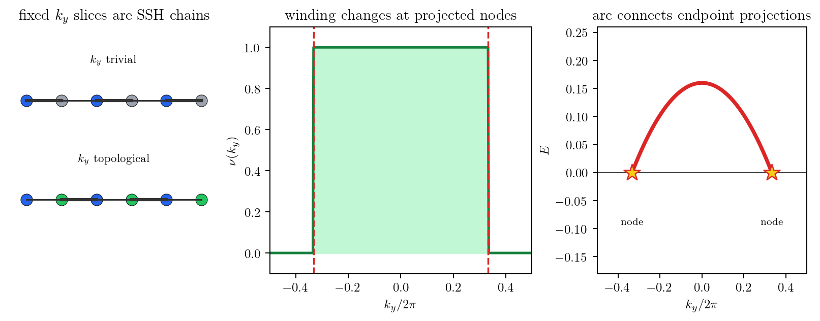
Figure 8.1: Cartoon of the Weyl/Majorana arc mechanism. Fixed (k_y) slices are SSH chains along (x). The winding changes across the projected Weyl nodes, and the paired boundary spectrum carries an arc connecting the endpoint projections.
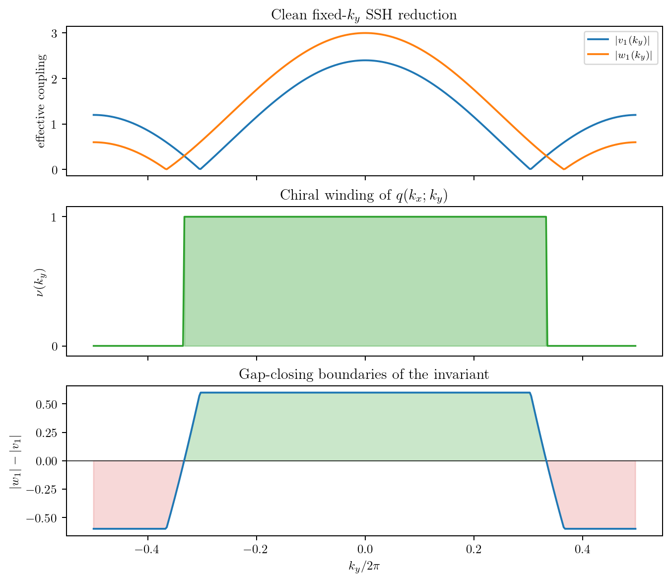
Figure 8.2: Clean bulk topology. For (\delta\epsilon=0), each (k_y) slice reduces to a chiral SSH chain along (x). The winding changes when the effective intracell and intercell hoppings exchange magnitude, predicting where the open-boundary Majorana arc should begin and end.
The imposed-pairing BdG problem uses an inter-sublattice cell pairing (\Delta_{AB}=\Delta_0), usually (\Delta_0=0.3), in the Nambu basis ((c_A,c_B,c_A^\dagger,c_B^\dagger)^T). The wall is a scalar onsite potential
where (W_\ell) is a one-cell-thick support of length (\ell). The wall is inside a periodic torus, not an imposed open boundary. The real-space plots use centered unit-cell coordinates, so the plotted wall is at (x=0). Unless stated otherwise, real-space densities are cell-resolved sums over the (A) and (B) sites in each unit cell.
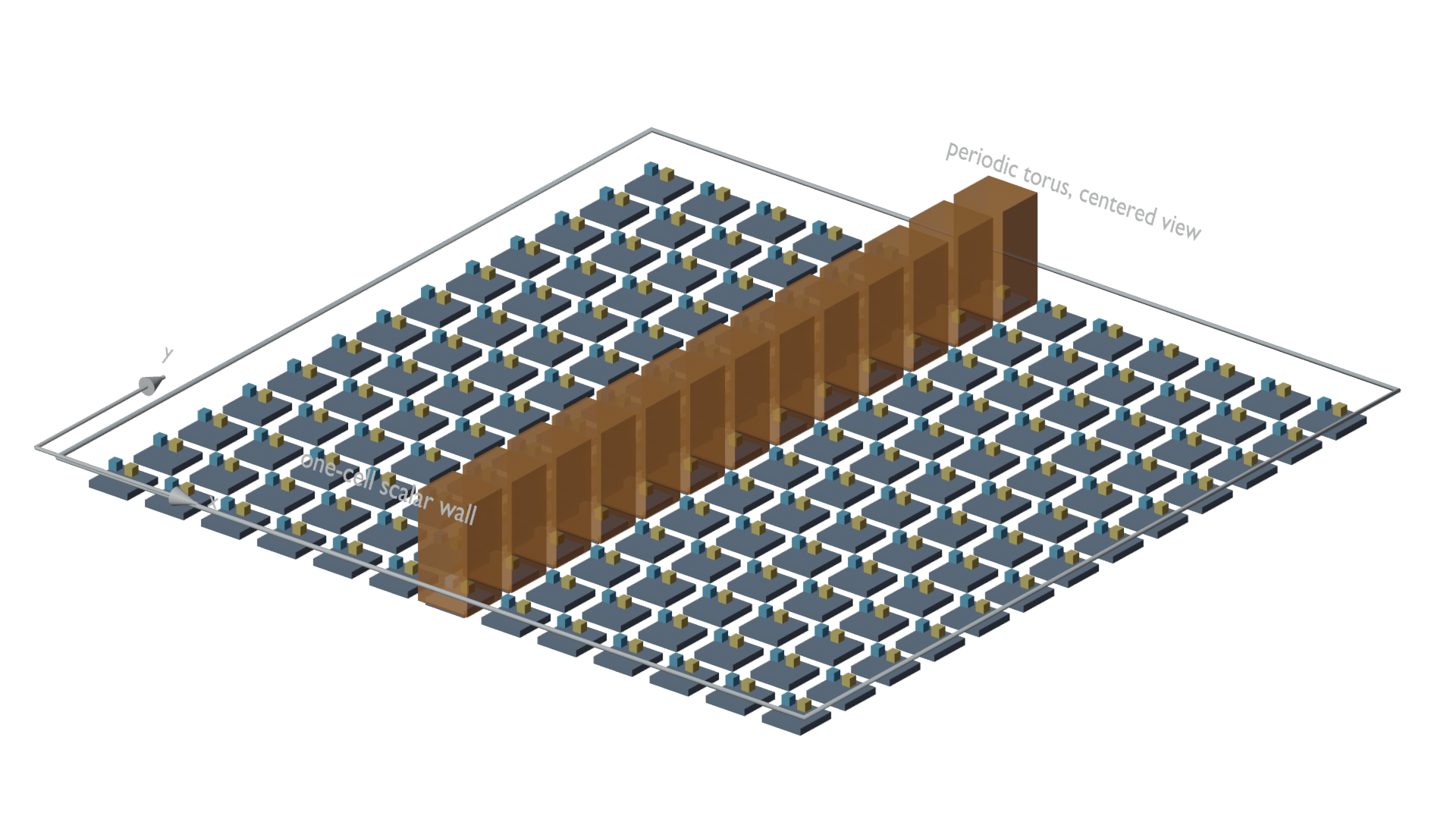
Figure 8.3: Three-dimensional view of the periodic wall setup. The orange cells mark the one-cell-thick scalar wall, the small blue and gold blocks show the two sublattice sites in each unit cell, and the compact axes indicate centered real-space coordinates. The render uses a (13\times13) representative lattice for clarity; the main fixed-pairing spectra and real-space diagnostics use (41\times41) unit cells unless stated otherwise.
The imposed-(\Delta_0) calculation isolates the quasiparticle boundary problem. For representative wall strengths, the wall-projected spectral function (A(k_y,E)) shows the boundary branch detach from the bulk response and approach the near-zero hard-wall arc.
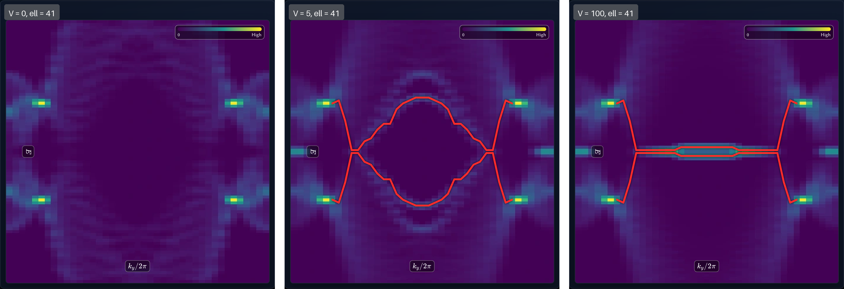
Figure 8.4: Viewer-exported wall-strength spectra for the imposed-pairing model on (41\times41) unit cells. The panels show (A(k_y,E)) at (\Delta_0=0.3), (\mu=\delta\epsilon=0), (\ell=41), and (V=0,5,100). The red curve follows the visible ADOS ridge and is clipped to the projected Weyl-node interval (|k_y|/2\pi\le 1/3).
To quantify the transfer, the calculation labels the branch by hard-wall ancestry rather than selecting a new local minimum at each parameter point. For each sampled (k_y), the tracker seeds the wall-weighted positive-energy mode at the largest simulated wall strength and continues that state downward in (V) by eigenvector overlap. When nearby eigenvalues have comparable single-vector overlaps, a small nearby-state subspace is used; ambiguous steps are logged and can be marked in the viewer. This makes the tracked branch a reproducible object, distinct from a purely visual ridge fit to (A(k_y,E)).
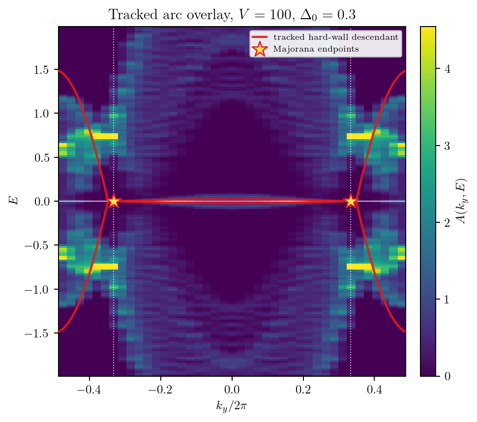
Figure 8.5: Tracked Weyl arc on top of the wall-projected spectrum. The background is (A(k_y,E)). The red curve is the hard-wall-descendant BdG branch selected by eigenvector and nearby-subspace overlap, and the yellow stars mark the clean Majorana endpoints at (k_y/2\pi=\pm 1/3).
The (k_y=0) point of the tracked branch provides a finite-size order parameter for the wall-driven transfer. Let (\epsilon_{\mathrm{arc}}(0;V)) be the wall-projected ADOS branch energy at (k_y=0), i.e. the distance from (E=0) to the selected positive-energy peak. The normalized order parameter is
In practice the hard-wall reference is represented by the largest simulated wall strength. The (41\times41) full-wall data show a sharp finite-device onset between (V=2.5) and (V=3). This is physically useful: it marks the wall strength where the tracked branch changes from a bulk-scale spectral feature into a hard-wall descendant. It is not reported as a critical point. Window scans of the Landau-style form
do not give a stable (V_c) or (\beta): fits that include the jump pin (V_c) to the first fitted point, while fits beginning after the jump drive (V_c) to an unphysical lower bound. A thermodynamic quantum-critical interpretation would require a size-scaling collapse of (\Psi_{\mathrm{arc}}(V,L)) and a consistent gap-closing diagnostic, neither of which is obtained from the present data.
Figure 8.6: Fixed-(\Delta_0) arc-transfer diagnostic. The left panel shows the tracked (k_y=0) arc energy as (V) is increased. The right panel shows (\Psi_{\mathrm{arc}}(V)). The data points use a full wall on a (41\times41) unit-cell device with (\Delta_0=0.3). The shaded band marks the finite-size onset window (2.5<V<3), not a fitted critical point.
The same transfer is visible in real space. The LDOS profiles below show wall-normal localization of selected spectral contributions at fixed (k_y) and energy. The component-resolved wavefunction shows the corresponding signed BdG amplitudes for the strong-wall near-zero mode. Together these diagnostics check that the tracked spectral branch is not merely a relabelled bulk eigenvalue.
In the BdG basis (\Psi=(c_A,c_B,c_A^\dagger,c_B^\dagger)^T), a wall eigenstate has spinor (\psi=(u_A,u_B,v_A,v_B)^T). Particle-hole symmetry pairs the state at energy (E) with a partner at (-E). At an exact Majorana zero mode the spinor can be gauge-fixed so that (v_\alpha=e^{i\phi}u_\alpha^\ast). The strong-wall state is therefore read as Majorana-like when the tracked branch approaches this particle-hole self-conjugate limit while remaining on the arc connecting the projected Weyl-node endpoints.
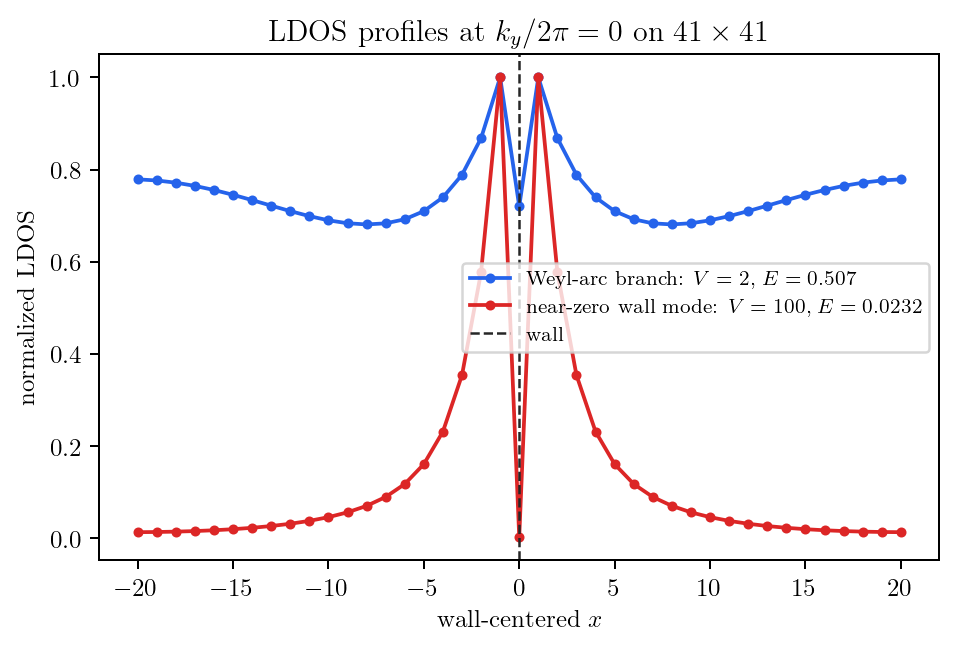
Figure 8.7: Wall-normal LDOS profiles on (41\times41) unit cells. The curves are evaluated at (k_y/2\pi=0): the Weyl-arc branch uses (V=2) and (E=0.507), while the near-zero wall mode uses (V=100) and (E=0.0232). Each curve is normalized by its own maximum, and the wall is marked at (x=0).
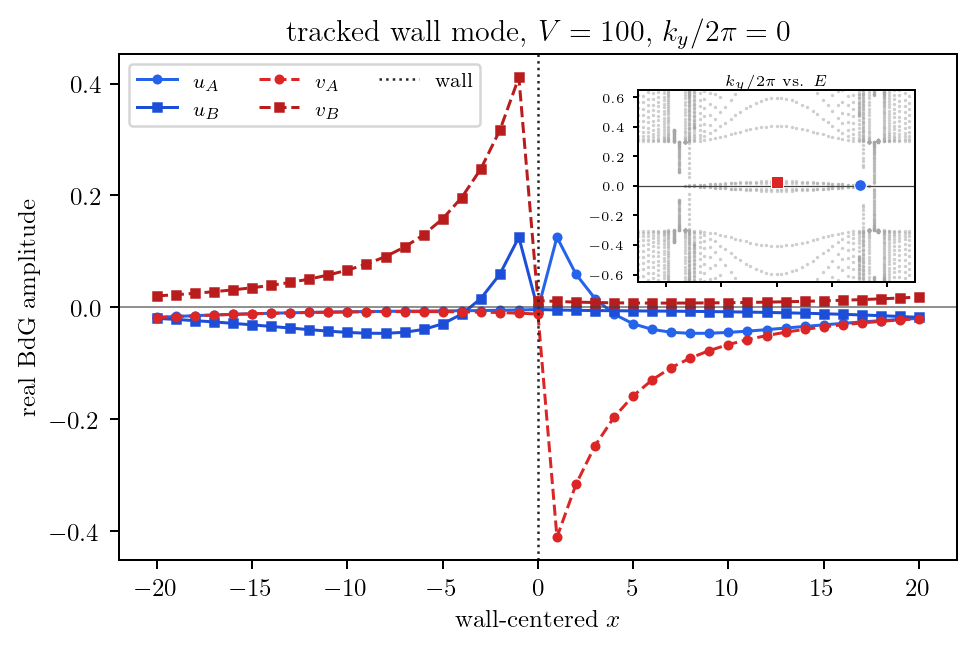
Figure 8.8: Component-resolved BdG wavefunction of the tracked strong-wall mode on (41\times41) unit cells. The curves show the real amplitudes ((u_A,u_B,v_A,v_B)) versus wall-centered (x) at (V=100), (k_y/2\pi=0), and (E=0.0232). The global phase is fixed by making the largest component real and positive.
The imposed calculation treats the wall as a scatterer in a fixed BdG background. The self-consistent calculation asks a stronger question: how does the anomalous field respond to the wall?
The interaction is decoupled through the local Gor’kov field
with the local mean-field pairing field
Here (\kappa_{AB}(r)) and (\Delta_{AB}(r)) are local inter-sublattice cell fields. The plots show (|\Delta_{AB}(r)|), or averages of this magnitude over wall and off-wall cell sets, so the displayed quantity is insensitive to the global sign convention for the real pairing gauge used in the calculation. This self-consistent field is distinct from the imposed constant (\Delta_0) used in the fixed-pairing BdG problem.
The self-consistent result is the main physical correction to the fixed-pairing picture. The wall is not only a scattering potential for quasiparticles. It also creates a local depression of the anomalous field: (|\Delta_{AB}(r)|) is strongly suppressed on the wall support while the off-wall condensate remains finite. Attempts to fit the wall mean to the same finite-(V_c) ansatz as the fixed-(\Delta_0) arc are unstable. The safer interpretation is wall-local depletion with an empirical algebraic tail over the simulated interval, with an exponent of order unity rather than a claimed critical exponent.
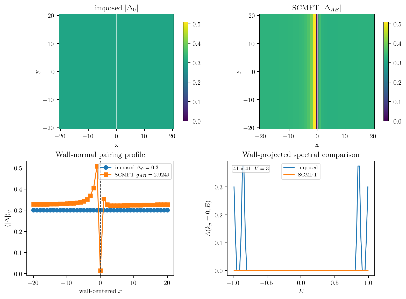
Figure 8.9: Direct fixed-pairing versus SCMFT comparison at the same wall. The imposed calculation keeps (|\Delta_0|) uniform, while the SCMFT solution suppresses the local (|\Delta_{AB}(r)|) at the wall and leaves the off-wall condensate finite.
| (V) | wall mean (|\Delta_{AB}|) | off-wall mean (|\Delta_{AB}|) | | —: | —: | —: | | 1.0 | 0.318 | 0.331 | | 1.1 | 0.234 | 0.329 | | 1.2 | 0.139 | 0.326 | | 1.3 | 0.0846 | 0.324 | | 1.5 | 0.0480 | 0.321 | | 2.0 | 0.0271 | 0.327 | | 3.0 | 0.0150 | 0.337 |
The clean winding invariant is exact only in the chiral slices of the translation-invariant model. The scalar onsite wall is a local chiral-symmetry-breaking perturbation because it contributes a same-sublattice onsite term on the wall cells. This does not invalidate the wall-transfer calculation; it clarifies what is being tested. The bulk away from the wall remains governed by the chiral SSH structure, while the wall locally breaks that symmetry and acts as a boundary-forming perturbation.
The local chiral marker is therefore used as a diagnostic, not as a final quantized invariant:
where (\Gamma=+1) on (A), (\Gamma=-1) on (B), and (Q=1-2P_-) is the flattened occupied-state projector. The comparison below shows that a scalar onsite wall and a chiral hopping cut are distinct boundary mechanisms.
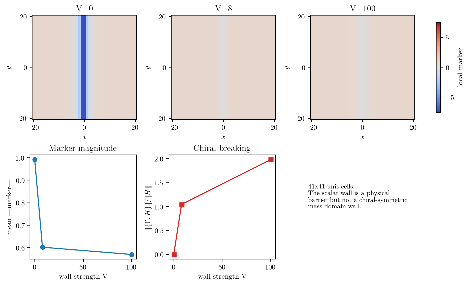
Figure 8.10: Local marker for the scalar onsite wall on (41\times41) unit cells. The bulk retains the clean chiral SSH structure, but the onsite impurity wall is a local chiral-symmetry-breaking defect.
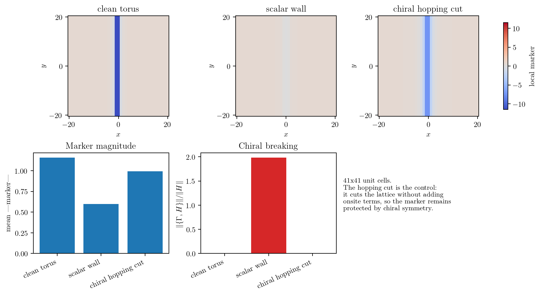
Figure 8.11: Chiral hopping-cut control on (41\times41) unit cells. This control changes inter-sublattice hopping terms rather than adding onsite potentials, showing that a scalar wall and a chiral-symmetric cut are distinct boundary mechanisms.
The current data support a finite-device arc-transfer crossover rather than a thermodynamic quantum critical point. The diagnostics below are kept in this chapter because they document the negative result: the onset can be sharp on a single device, but the fitted exponent and finite-size onset do not stabilize.
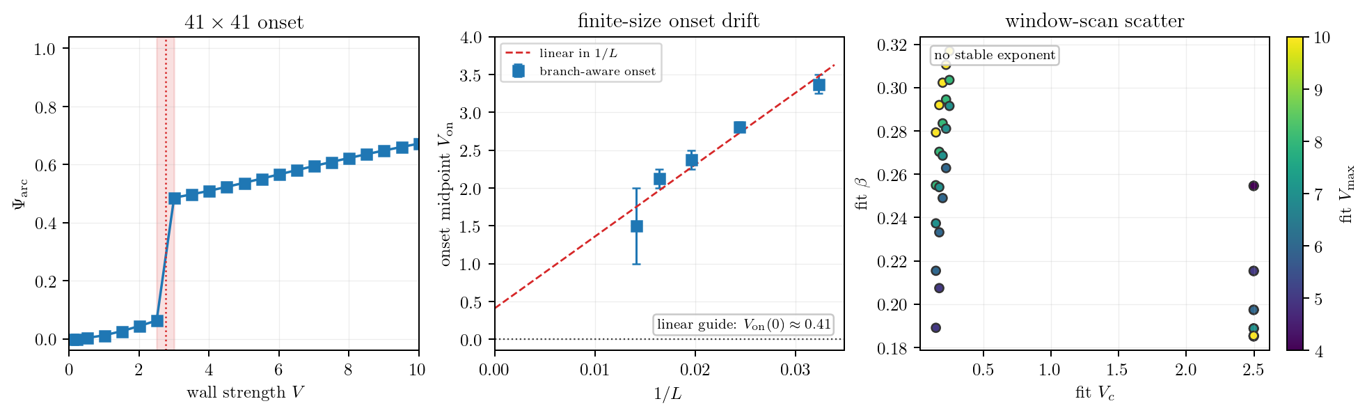
Figure 8.12: Finite-size checks for a possible critical interpretation of the arc-transfer onset. The (41\times41) order parameter has its largest jump between (V=2.5) and (V=3), but the branch-aware emergence onset drifts with increasing (L), and the fit-window scan does not give a stable cluster of (V_c) and (\beta).
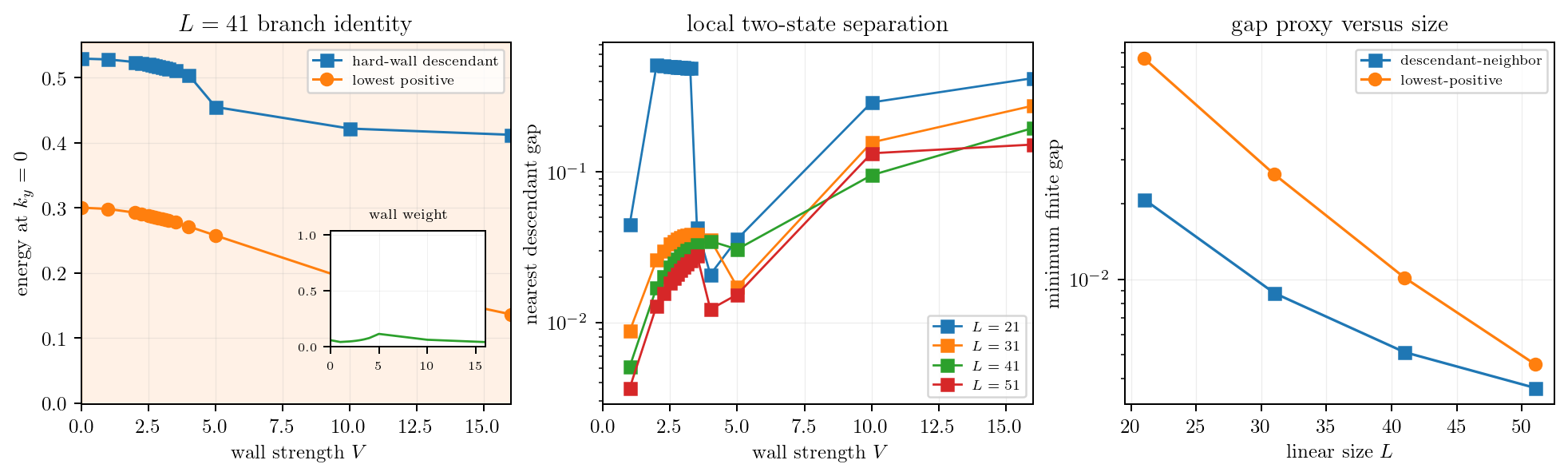
Figure 8.13: Fixed-(k_y) two-state diagnostic for the arc-transfer onset. The hard-wall descendant and the lowest positive-energy wall state are usually distinct at (k_y=0), so the visible ADOS/eigenvalue onset and the hard-wall-descendant tracker need not label the same spectral feature.
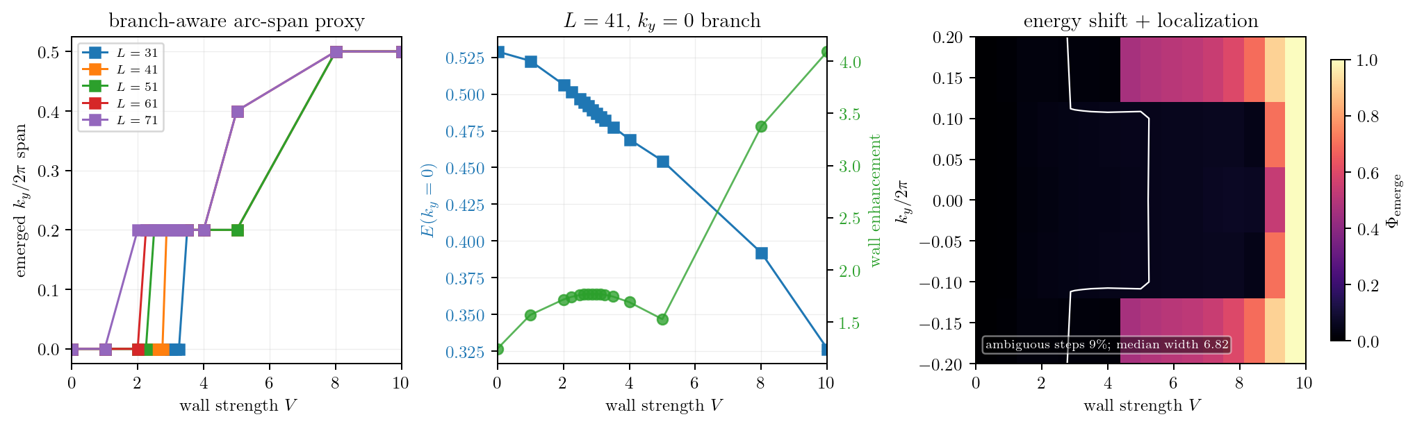
Figure 8.14: Branch-aware bulk-emergence diagnostic for the arc-height order parameter. The scan repeats the wall-enhanced branch selection over several (k_y) slices for (L=31,41,51,61,71). The onset proxy drifts downward with increasing size rather than defining a size-stable finite (V_c).
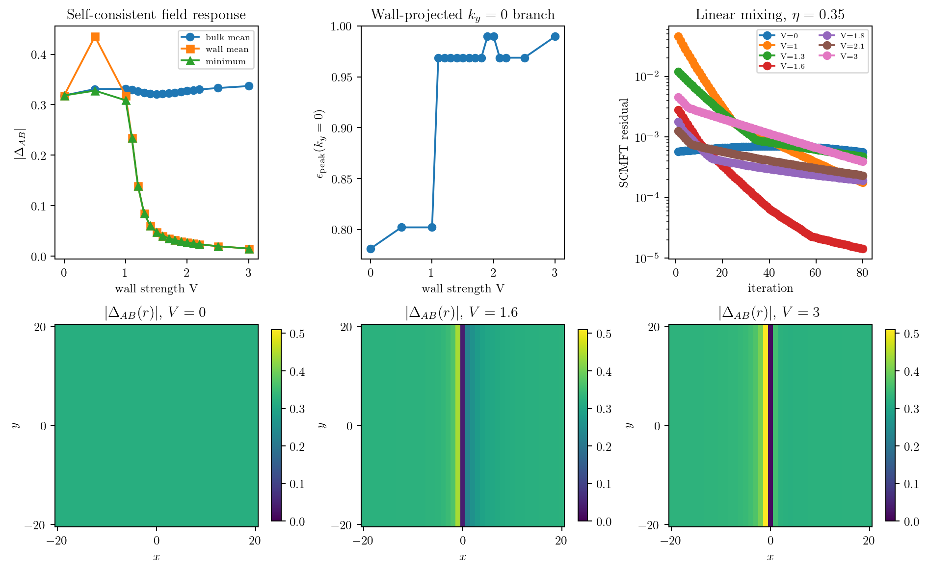
Figure 8.15: Self-consistent mean-field wall response. The field maps and convergence histories show that the wall suppresses the local Gor’kov field and expels the pairing amplitude from the wall support while the off-wall condensate remains finite.
Soft impurity walls provide a controlled finite-device route from clean momentum-space topology to a real-space internal boundary in a superconducting SSH lattice. In the fixed-(\Delta_0) problem, the (k_y=0) branch begins as a bulk-scale spectral feature and moves toward the near-zero hard-wall branch as (V) grows. In the self-consistent problem, the same wall suppresses (\kappa_{AB}(r)) and (\Delta_{AB}(r)) on the wall support while preserving a finite off-wall condensate.
The conservative conclusion is a linked chain of evidence: clean slice winding, slab Majorana arcs, wall-projected spectral evolution, eigenvector-continuous arc tracking, real-space mode localization, and self-consistent suppression of the wall pairing field. The current evidence does not justify a reported critical exponent. A stronger quantum-critical claim would require stable finite-size scaling of the order parameter and the relevant quasiparticle gap, performed on the same selected states. Until then, the result is a sharp and useful finite-device onset of Weyl-arc transfer, not an identified thermodynamic phase transition.
Numerical data and figures were generated with the qulab.research.ssh_2d
module in QuLab [13].
Paper 1 established a microscopic loop-supercurrent route to time-reversal symmetry breaking (TRSB) by branch ranking in a current-channel BdG closure, with strict winding/circulation filters and a triplet-penalty decomposition. The objective here is a narrower continuation question: starting from a loop-favored winding texture, what transition structure is implied when the normal-state sector is extended by Rashba spin–orbit coupling and Zeeman splitting?
Within the full thesis hierarchy, this chapter should be read as an effective topological sidecar rather than as a literal materials model. Its role is to ask what kinds of class-D topological structure can be induced once a TRSB superconducting texture has already been selected microscopically. The later LaNiX materials chapter is where the normal-state Hilbert space is earned from crystallography, DFT, and Wannierization. The present chapter instead probes a reduced orbital block that is best interpreted as a topology-facing descendant of that programme, especially on the LaNiGa side where nonsymmorphic low-energy structure and boundary physics are part of the materials motivation.
This manuscript is intentionally scoped as an analytic-first topological probe (Tier 1). Its central deliverable is an explicit mass-inversion transition fan at the time-reversal invariant momenta (TRIM) and a corresponding piecewise-constant proxy index. Numerical results are deliberately restricted to targeted confirmations (representative bulk band cuts and strip spectra) across a matched proxy transition. We do not present full two-parameter Chern/gap heatmaps here.
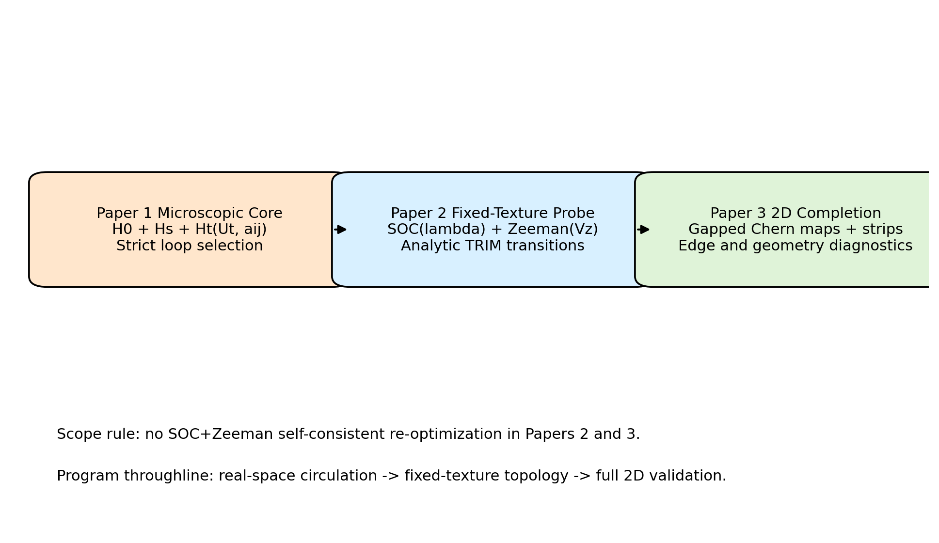
Program hierarchy from microscopic loop selection to fixed-texture topological probing and full 2D completion. Paper 1 supplies the branch-selected winding baseline; this paper (Tier 1) adds SOC+Zeeman at fixed texture and reports analytic TRIM transitions with targeted spectral checks; full 2D Chern/gap maps are deferred to Paper 3.
Additional diagnostic (real-space topology in open geometry). In open-boundary settings, topology can be monitored using local real-space markers built from projectors (local Chern marker) and their associated redistribution/flow (“marker currents”). We do not study non-equilibrium marker-current dynamics here; we include only a static local-marker visualization as a companion to the strip spectrum.
To keep claims clean, we separate three layers:
The paper-1 Hamiltonian is
\begin{equation} H = H_0 + H_s + H_t, \end{equation} with onsite singlet pairing field
\begin{equation} \Delta_i = U_s\langle \hat c_{i\downarrow}\hat c_{i\uparrow}\rangle, \end{equation} and current-channel HS saddle
\begin{equation} a_{ij}=U_t\langle \hat J_{ij}\rangle,\qquad \hat J_{ij}=it\sum_\sigma(\hat c^\dagger_{i\sigma}\hat c_{j\sigma}-\hat c^\dagger_{j\sigma}\hat c_{i\sigma}). \end{equation} Branch ranking in paper 1 used
\begin{equation} F_{\rm eff}=F_{\rm BdG}+\Chi_{\rm trip}^{\rm edge}+\Chi_{\rm trip}^{\rm diag}, \end{equation} with strict loop acceptance criteria (e.g., (\Delta F_{\rm eff}<0), winding index (m=\pm1), circulation coherence).
[Insert paper-1 anchor figures with explicit provenance.]
We add spinful SOC+Zeeman terms to the normal block while keeping a winding pairing texture motivated by the paper-1 loop branch.
\begin{equation} h_{\rm topo}(\mathbf{k}) = h_{\rm orb}(\mathbf{k})\otimes\sigma_0 + \lambda(\sin k_y,\sigma_x-\sin k_x,\sigma_y) + V_z\sigma_z, \end{equation}
with (\sigma_i) acting in spin space and (h_{\rm orb}(\mathbf k)) the orbital tight-binding block (parameters stated in figure captions and run logs).
Optional flux decoration (kept OFF in this paper). A natural multi-orbital extension is to allow Peierls phases on selected hoppings to represent engineered flux patterns in the orbital block. We define the bookkeeping for this extension (to keep codepaths consistent with Paper B), but set the flux parameter (\Phi=0) throughout Paper A.
\begin{equation} \mathcal H_{\mathrm{BdG}}(\mathbf k)= \begin{pmatrix} h_{\rm topo}(\mathbf k) & \Delta \ \Delta^\dagger & -h_{\rm topo}^T(-\mathbf k) \end{pmatrix}. \end{equation}
The particle sector has dimension (4\times2=8) (orbital (\times) spin) and the full BdG matrix is (16\times16).
Pairing is onsite singlet and orbital-diagonal with a fixed intracell winding pattern
\begin{equation} (\Delta_A,\Delta_B,\Delta_C,\Delta_D) = \Delta_0(1,e^{i\pi/2},e^{i\pi},e^{i3\pi/2}). \end{equation}
This texture is imposed (seeded from the loop program) and not re-optimized under SOC+Zeeman.
Native QTT geometry view of the fixed-texture Topo-BdG unit cell used in this Tier-1 probe. The figure is generated directly from the canonical shared model definition, making the plaquette basis and hopping graph explicit without introducing extra hand-drawn conventions.
We fix a single set of conventions for all reported spectra, proxy indices, and (optional) Chern/marker checks.
Real-space unit cell and orbital order. Each Bravais cell contains four orbitals in the order
\begin{equation} (A,B,C,D)\equiv (0,0),(1,0),(0,1),(1,1), \end{equation} and the Bloch orbital spinor is
\begin{equation} \hat c_{\mathbf k}=\big(\hat c_{\mathbf k,A},\hat c_{\mathbf k,B},\hat c_{\mathbf k,C},\hat c_{\mathbf k,D}\big)^T. \end{equation}
Brillouin-zone orientation and integration convention. We use ((k_x,k_y)\in[-\pi,\pi)\times[-\pi,\pi)) with the standard right-handed orientation. Whenever a Chern sign is referenced (e.g. for optional selected-point validation), it is computed with the oriented area element (dk_x\wedge dk_y). TRIM are ordered as (\Gamma=(0,0), X=(\pi,0), Y=(0,\pi), M=(\pi,\pi)).
High-symmetry path direction. Band plots use the directed path (\Gamma\to X\to M\to \Gamma) (unless explicitly stated otherwise in the caption/run log).
Spin and Nambu (BdG) basis ordering. The spinful particle basis is ordered as
\begin{equation} \hat c_{\mathbf k}= \big(\hat c_{\mathbf k,A\uparrow},\hat c_{\mathbf k,A\downarrow}, \hat c_{\mathbf k,B\uparrow},\hat c_{\mathbf k,B\downarrow}, \hat c_{\mathbf k,C\uparrow},\hat c_{\mathbf k,C\downarrow}, \hat c_{\mathbf k,D\uparrow},\hat c_{\mathbf k,D\downarrow}\big)^T. \end{equation} The Nambu spinor is
\begin{equation} \Psi_{\mathbf k}=\big(\hat c_{\mathbf k},,\hat c^\dagger_{-\mathbf k}\big)^T, \end{equation} so (\mathcal H_{\rm BdG}(\mathbf k)) is (16\times16).
Sign-sensitive labels. Winding-like labels and some sign conventions can flip under equivalent relabelings (orbital permutations, unit-cell embedding changes, or altered symmetry-operator phases). We therefore treat signs as declared conventions and keep them fixed across all scripts and figures.
The time-reversal invariant momenta (TRIM) are the four points (K) satisfying (K=-K) modulo reciprocal lattice vectors. For a square lattice:
\begin{equation} \Gamma=(0,0),\quad X=(\pi,0),\quad Y=(0,\pi),\quad M=(\pi,\pi). \end{equation}
Gap closings at these points control a clean analytic transition structure.
Let (\epsilon_n(K,\mu)) be eigenvalues of (h_{\rm orb}(K)). Define the TRIM mass
\begin{equation} m_{n,K}(\mu,V_z) = V_z^2-\left(\epsilon_n(K,\mu)^2+\Delta_0^2\right). \end{equation} Candidate transition lines (“fan”) are
\begin{equation} V_z=\sqrt{\epsilon_n(K,\mu)^2+\Delta_0^2}. \end{equation}
Assign chirality weights
\begin{equation} \eta_\Gamma=\eta_M=+1,\qquad \eta_X=\eta_Y=-1, \end{equation} and define
\begin{equation} C_{\rm proxy}(\mu,V_z)=\frac12\sum_{n,K}\eta_K\left[\mathrm{sgn}(m_{n,K})-\mathrm{sgn}(m_{n,K}|_{V_z=0})\right]. \end{equation} This index is a proxy: it is intended to organize candidate transitions associated with TRIM mass inversions. It does not replace a full 2D Chern evaluation away from TRIM.
In class D, a gapped phase with integer (C) supports (|C|) chiral Majorana edge modes (with sign fixed by orientation convention), so the proxy is used only to pre-organize where this edge content can change through a bulk gap closing. Conceptually, this continuation keeps a common circulation thread: real-space loop circulation in paper 1, order-parameter winding in the fixed texture, and momentum-space Berry-curvature circulation in the topological sector.
[Insert fig_code_03_analytic_chern_proxy_map_01.png and cite the generated CSV analytic_chern_proxy_map.csv.]
Captions must state grid sizes and all parameter values used.
We select a representative chemical potential and SOC strength (stated in the figure caption/run log) and plot bulk BdG dispersions along a standard high-symmetry path (e.g., (\Gamma!!-!X!!-!M!!-!\Gamma)) at two Zeeman fields straddling the first proxy line.
[Insert fig_code_04_bulk_bands_analytic_transition_cut_01.png.]
In-panel text reports a mesh-estimated minimum gap (\min_{\mathbf k} E_{\min}(\mathbf k)).
We compute strip spectra (open (x), periodic (k_y)) at two Zeeman fields bracketing the same proxy transition and color eigenvalues by an explicit edge-localization weight.
[Insert fig_code_05_bulk_boundary_correspondence_01.png and cite bulk_boundary_correspondence_summary.txt.]
At the same strip parameters, we optionally compute a static local marker built from the occupied-state projector in the open geometry, yielding a spatial profile that distinguishes bulk-like regions from boundary reconstructions. This is included solely as a companion visualization alongside the edge-weight strip spectrum.
[Optional insert fig_code_05b_local_chern_marker_strip_01.png and cite local_marker_strip_summary.txt.]
We introduced an analytic TRIM mass-inversion construction for a fixed-texture SOC+Zeeman extension seeded from a loop/TRSB winding pattern, yielding an explicit transition fan and a piecewise-constant proxy index. Representative bulk and strip diagnostics support spectral reorganization and bulk–boundary contrast across a matched proxy transition, with an optional static local-marker companion in open geometry. This provides an analytic-first organizing framework and a concrete continuation target for a subsequent referee-proof 2D topological characterization.
../microscopic-loop-supercurrent-trsb/index.md.This chapter extends the same symmetry and tensor-product structure used for quadratic, free-fermion, and BdG models to quartic, two-body lattice Hamiltonians. The aim is to write the most general interacting Hamiltonian consistent with the physical structure of the problem: lattice translations, boundaries, inhomogeneous geometries, and defects implemented through masks; Nambu doubling when it is useful for pairing-channel bookkeeping and later mean-field decouplings; internal structure such as sublattices, orbitals, and intra-cell positions; spin; and the chosen set of symmetry generators.
The organising principle is that quartic Hamiltonians may be constructed systematically as symmetry-constrained combinations of products of bilinears, where each bilinear is the second-quantized lift of a single-particle operator written in the same tensor-product order as in the quadratic chapter. In this way, the interacting theory remains compatible with later mean-field reductions: once an interaction has been specified, the admissible quadratic orders are precisely the symmetry-allowed bilinears that can appear as decoupling channels.
From the condensed-matter side, this is the natural language in which on-site Hubbard interactions, extended density-density couplings, and multiorbital local interactions are usually formulated before one chooses a particular approximation scheme or pairing channel. [14, 15, 16, 17]
We keep the same single-particle tensor-product order
When Nambu space is absent, that factor is omitted.
Define a composite internal index
and write fermion operators as
with the same intra-cell position-phase convention as in the quadratic chapter if desired.
Given any single-particle operator (X) acting on (\mathcal H) (in the fixed tensor order), define its many-body (second-quantized) lift
where (m,n) range over the full one-particle basis (site ⊗ internal ⊗ spin, and Nambu if used).
This construction provides the bridge between the quadratic and quartic theories. Quadratic Hamiltonians are sums of operators of the form (\widehat X), whereas quartic Hamiltonians are built from products of such operators, typically in normal-ordered form.
A symmetry-compatible and nonredundant container for many interactions is
with Hermitian (X_\mu) and a real symmetric coupling matrix (g_{\mu\nu}=g_{\nu\mu}) (after choosing a Hermitian operator basis). Normal ordering removes the quadratic “Hartree” pieces from the algebraic definition, so that quadratic terms are handled in the quadratic chapter and quartic terms remain genuinely interacting.
Accordingly, the operators (X_\mu) should already respect the lattice structure, including shifts, masks, and boundaries, while symmetry acts on the remaining tensor factors.
Retain the mask ( \mathbb M ) on (\mathcal H_{\text{lat}}) and the masked shift
For interactions it is often convenient to also use site projectors on lattice space:
These give a clean “operator density at (\mathbf R)” construction.
Let (\Gamma) be any Hermitian matrix acting on (\mathcal H_{\text{(Nambu)}}\otimes\mathcal H_{\text{int}}\otimes\mathcal H_{\text{spin}}). Define the local bilinear (operator density) at (\mathbf R)
Equivalently, (\widehat O_\Gamma(\mathbf R)=\widehat X) with
Common choices of (\Gamma) include the charge-density channel (\Gamma=\mathbb 1), the spin-density channels (\Gamma=\sigma_j), the orbital-density channels (\Gamma=\lambda_i), and, when Nambu space is retained, combined channels of the form (\Gamma=\tau_\ell\otimes\lambda_i\otimes\sigma_j).
A large class of lattice interactions can be written as sums over displacements (\boldsymbol\delta\in\mathcal D):
This is the interacting analogue of restricting a quadratic model to a finite displacement set (\mathcal D).
Masking is implemented by restricting (\mathbf R) to active sites (or inserting (m_{\mathbf R}m_{\mathbf R+\boldsymbol\delta}) in the sum).
Special cases include the on-site Hubbard interaction, obtained with (\boldsymbol\delta=\mathbf 0) and (\Gamma) chosen to resolve the spin densities, or directly as (Un_{\uparrow}n_{\downarrow}); nearest-neighbour density interactions, for which (\Gamma=\mathbb 1) and (|\boldsymbol\delta|=a); spin-exchange terms with (\Gamma=\sigma_j) and (|\boldsymbol\delta|=a); and orbital-exchange or Kugel-Khomskii-type structures involving (\Gamma=\lambda_i) and (\Gamma=\lambda_i\otimes\sigma_j).
In this formulation, the lattice geometry is encoded in (\mathcal D) and (\mathbb M), while the (\Gamma)-structure is treated as internal, spin, and, when present, Nambu algebra subject to symmetry.
The interaction classes most relevant to the present thesis are those that lead naturally to superconducting, bond-resolved, and multiorbital mean-field channels. The general quartic framework becomes concrete in the following examples.
Schematic interaction channels on a lattice. The central local process represents an on-site interaction between opposite-spin electrons occupying the same orbital, as in the attractive or repulsive Hubbard term; the label marks this local singlet channel. The right-hand process indicates a finite-range bond-resolved channel, where interactions couple neighboring sites; the label marks a nonlocal triplet channel that can naturally generate exchange, bond-order, current, or nonlocal pairing decouplings in the mean-field reduction.
The simplest superconducting example is the on-site attractive Hubbard interaction [14, 15]
In the present formalism this is an on-site quartic term, corresponding to (\boldsymbol\delta=\mathbf 0), and it is the natural starting point for on-site spin-singlet pairing. Decoupling in the anomalous channel gives
so that the resulting quadratic theory contains terms of the form
together with the corresponding Hartree shifts. This is the minimal interaction underlying the lattice BdG constructions used later in the thesis and the standard microscopic bridge to the BCS/Gor’kov mean-field description. [18, 19]
A second important class consists of finite-range density interactions such as
This is the simplest example with a nontrivial displacement set (\mathcal D), and therefore makes explicit contact with the harmonic structure discussed above. In the superconductivity literature this is the standard extension beyond the on-site Hubbard term when one wants nonlocal charge, bond, or pairing channels. [15, 20, 21] On the square lattice one obtains
so the interaction already carries the lattice harmonics that later distinguish different ordering patterns. Decoupling in the particle-hole sector can favour charge order, whereas decoupling in the bond-singlet pairing sector gives
The symmetry of the bond pattern then distinguishes extended (s)-wave from (d_{x^2-y^2})-type pairing. This example is therefore the direct interacting analogue of the finite-displacement quadratic models discussed in the preceding chapter.
The loop-supercurrent chapters are naturally connected to interactions written in terms of bond-current operators. For an oriented bond (b=(\mathbf R,\mathbf R’)), define
A quartic current-channel interaction may then be written as
In the bilinear-product language, this is simply a coupling between bond bilinears rather than on-site densities. A mean-field decoupling introduces bond fields
which enter the quadratic Hamiltonian as directed bond terms, or equivalently as self-consistent imaginary hopping amplitudes. It is in this sense that current-channel interactions provide a microscopic route to time-reversal-breaking loop-current or loop-supercurrent states, including the loop-supercurrent constructions discussed later in the thesis. [22]
When several orbitals or sublattices are retained inside the same unit cell, local interactions acquire a richer internal structure. The standard local multiorbital parametrization goes back to Kanamori, while the corresponding spin-orbital exchange descendants are often summarized as Kugel-Khomskii-type interactions. [16, 17] A standard multiorbital form is
written here for a single site or unit cell with orbital labels (a,b). Such terms are naturally expanded in the (\lambda_i\otimes\sigma_j) basis introduced above. They can generate orbital polarisation, spin exchange, interorbital singlet pairing, or more specialised multicomponent pairing penalties and couplings. This is precisely the class of interaction structure needed once internal degrees of freedom inside a unit cell become central to the later microscopic superconducting models.
In a general basis label (p=(\mathbf R,\alpha)) (or ((\mathbf k,\alpha)) in momentum space),
Fermion statistics and Hermiticity impose antisymmetry in the incoming legs,
antisymmetry in the outgoing legs,
and Hermiticity,
The bilinear-product container ( \sum g_{\mu\nu}:\widehat X_\mu\widehat X_\nu: ) is a structured way to parameterize such (V) while keeping symmetry constraints tractable.
Assume periodic boundaries and (\mathbb M=\mathbb 1). Translation invariance implies momentum conservation (up to a reciprocal lattice vector (\mathbf G)):
A common reduced parametrization uses transfer momentum (\mathbf q):
If in real space you kept a finite displacement set (\mathcal D), then the (\mathbf q)-dependence is a finite harmonic expansion:
where each (V_{\boldsymbol\delta}) is a matrix in the internal/spin (and possibly Nambu-channel) indices.
This is the interaction analogue of the quadratic “Bloch polynomial” in (\mathbf k).
Let a unitary spatial symmetry (g) act on the one-particle Hilbert space by
with (U_g(\mathbf k)) constructed exactly as in the quadratic chapter:
When Nambu space is absent, the factor (U_g^{(\text{Nambu})}) is omitted.
Time reversal (\mathsf T) (antiunitary) acts as
i.e. complex conjugation in coefficients plus the unitary matrix (U_{\mathsf T}) on internal/spin (and possibly Nambu) indices.
In momentum space, invariance under a unitary symmetry (g) imposes
together with momentum conservation.
For time reversal (\mathsf T),
These are the direct interacting analogues of the quadratic constraints (U_g,\mathcal H(\mathbf k),U_g^\dagger=\mathcal H(g\mathbf k)) and (U_{\mathsf T},\mathcal H(\mathbf k)^*,U_{\mathsf T}^\dagger=\mathcal H(-\mathbf k)), but now acting on a rank-4 vertex.
If the interaction is written as
and the symmetry maps the basis by
then invariance is the matrix condition
For antiunitary symmetries, include complex conjugation of coefficients; with a Hermitian basis one typically works with real (g) after enforcing constraints.
In practice, one computes (R_g) by acting with (U_g) on the single-particle operators (X_\mu), and then enforces (g=R_g g R_g^T) as a system of linear constraints.
As in the quadratic chapter, one chooses Hermitian bases ({\tau_\ell}) for Nambu space when it is present, ({\lambda_i}) for the internal sector, and ({\sigma_j}) for spin.
Define channel matrices
Then local bilinears are
and finite-range interactions can be expanded as
Symmetry constraints act only on the index structure ((\ell,i,j)) and on the displacement classes (\boldsymbol\delta) (or their orbits under the point group), exactly mirroring the quadratic form-factor selection.
A quartic term written as a product of bilinears provides an immediate mean-field/Hubbard–Stratonovich entry point:
with an analogous construction for pairing-type decouplings when Nambu space is retained.
Two consequences follow. First, the allowed order parameters are precisely the symmetry-allowed bilinears: the generator constraints of the quadratic chapter determine which (\widehat O_\mu) may acquire expectation values without explicitly breaking the imposed symmetries. Second, the question of competition or coexistence among candidate orders is inherited from the symmetry-allowed invariants. Once a set of channels ({\widehat O_\mu}) has been selected, the Landau-type couplings among the associated mean fields are constrained by the same generator logic, with coefficients determined in principle by the microscopic couplings (g_{\mu\nu}).
Mean-field terms should therefore not be introduced independently, but obtained by decoupling a symmetry-allowed quartic Hamiltonian in symmetry-identified channels. This is the same logic that underlies standard superconducting mean-field theory, microscopic derivations of Ginzburg-Landau theory, and symmetry-based Landau expansions of unconventional order parameters. [23, 19, 24, 25]
The construction proceeds in a natural sequence. One first fixes the lattice structure by specifying the lattice shape (\mathbf N), the boundary conditions, the mask (\mathbb M), and a finite displacement set (\mathcal D). One then chooses a bilinear operator basis of the form
with (\Gamma_\mu) drawn from (\tau\otimes\lambda\otimes\sigma), or from (\lambda\otimes\sigma) when Nambu space is absent. The quartic Hamiltonian is then written in the container
or, equivalently, in a displacement-resolved form with couplings (g^{(\boldsymbol\delta)}).
At that stage one imposes the intrinsic fermionic constraints, namely antisymmetry and Hermiticity, either directly on the vertex (V) or implicitly through the use of Hermitian bilinear bases and symmetric coupling matrices (g). The next step is to construct the generator representations (U_g(\mathbf k)) exactly as in the quadratic chapter, including the intra-cell phase conventions, and from these obtain the induced action (R_g) on the basis (X_\mu). Solving the resulting linear constraints, (g=R_g g R_g^T) together with the antiunitary variants, yields the most general symmetry-allowed coupling space.
If desired, this space may then be organised further by projection into irreducible representations of the point group or spin-rotation group, and may subsequently be reduced by controlled approximations such as mean-field decoupling, random-phase approximation, or functional-renormalization-group truncations.
A symmetry-compatible quartic model can be written as
with generator constraints implemented as
and with translation invariance giving momentum conservation plus finite-harmonic (\mathbf q)-dependence when the interaction range is finite.
Muon-spin-relaxation experiments report time-reversal-symmetry breaking in both noncentrosymmetric LaNiC(_2) and centrosymmetric LaNiGa(_2) [26, 27]. Thermodynamic probes also indicate multigap, largely nodeless superconductivity [28, 29]. Internally antisymmetric nonunitary triplet (INT) pairing was proposed to reconcile these facts by combining equal-spin triplet structure with an antisymmetric orbital label [27, 28, 30].
The chapter asks a narrower question than the phenomenology. If the INT gap is imposed, the algebraic and spectral signatures are straightforward. The nontrivial test is whether a controlled microscopic mean-field calculation selects that nonunitary branch over singlet, unitary triplet, mixed, or normal alternatives. The result is a benchmark, not an exclusion theorem: under the local Hubbard-Kanamori-like assumptions and survey-quality LaNiX(_2) Hamiltonians tested here, robust spontaneous nonunitary INT order is not obtained.
The minimal toy model uses two active orbitals (a,b) and spin. In the basis ((c_{a\uparrow},c_{a\downarrow},c_{b\uparrow},c_{b\downarrow})), the normal Hamiltonian is
For the retained two-dimensional figures,
Here (t) sets the hopping scale, (\mu) is the chemical potential, (s) is the orbital splitting, (v_0,v_1) are interorbital hybridisations, and the baseline spin-orbit term is longitudinal with respect to the chosen (\uparrow/\downarrow) quantization axis. Projection-repair scans additionally allow transverse texture terms such as (\lambda_x\tau_y\sigma_x).
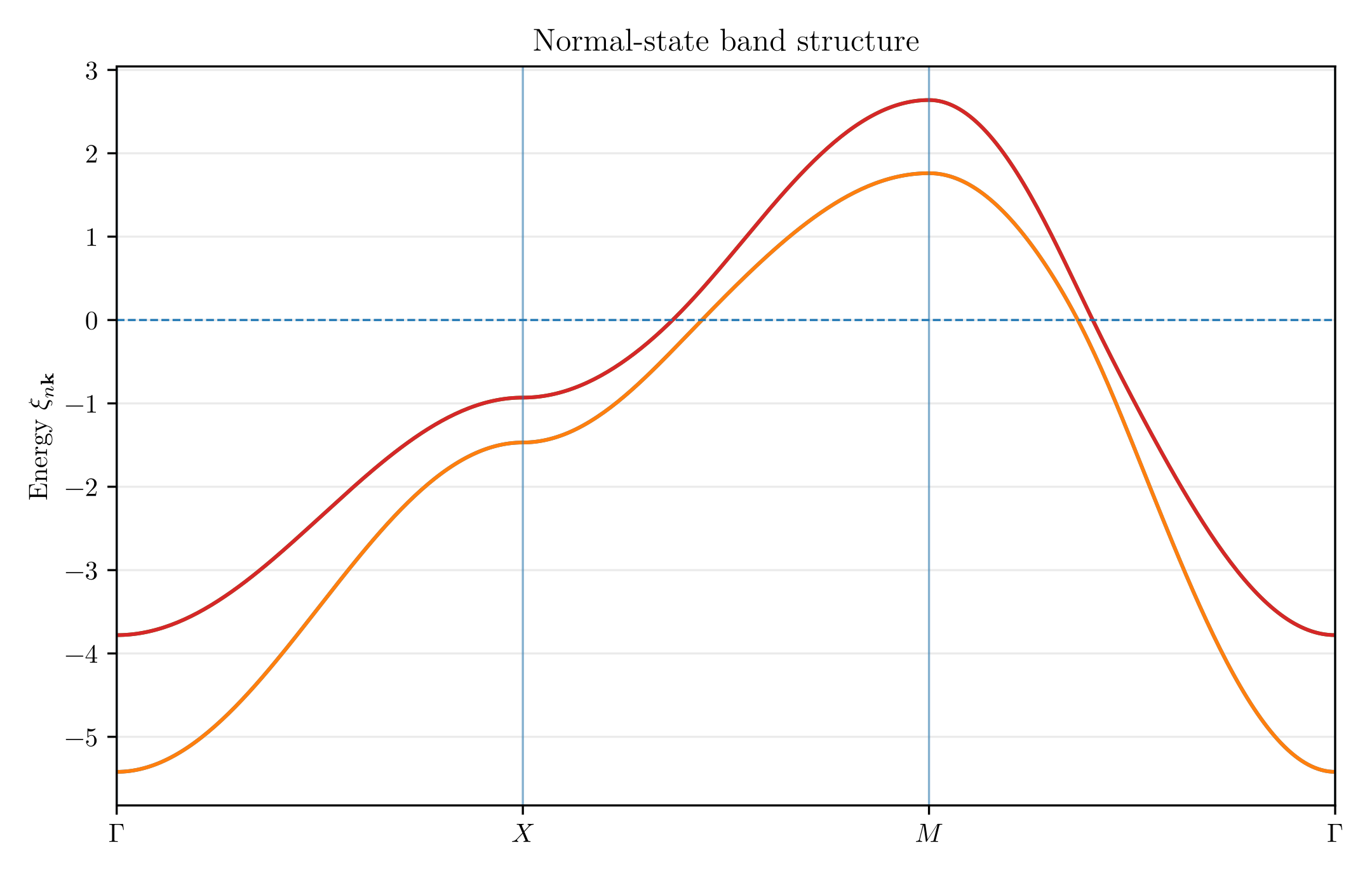
Figure 8.16: Normal-state band structure for the two-orbital toy model.
The local interaction is the two-orbital Hubbard-Kanamori form [16],
with
Positive (U,U’,J_H,J_P) denote repulsive microscopic parameters. With the exchange operator ordered as above,
so the equal-spin interorbital triplet scale is
Hund exchange lowers the equal-spin interorbital triplet channel relative to interorbital singlet competitors. That is not the same as proving a superconducting instability: for ordinary repulsive parameters the INT channel may be the least repulsive descendant without being attractive unless the effective vertex is renormalized or supplied phenomenologically.
The inverse scalar pairing susceptibility is defined by the channel kernel
where (\chi_\alpha) is the normal-state pair susceptibility projected onto channel (\alpha), and (\mathbf U_\alpha) is the relevant component of the local interaction tensor. Equivalently, the plotted dimensionless eigenvalues are
for which (\lambda_\alpha=1) is the scalar linearized instability condition. For the retained diagnostic, the toy susceptibilities are held fixed at (T=0.05), while
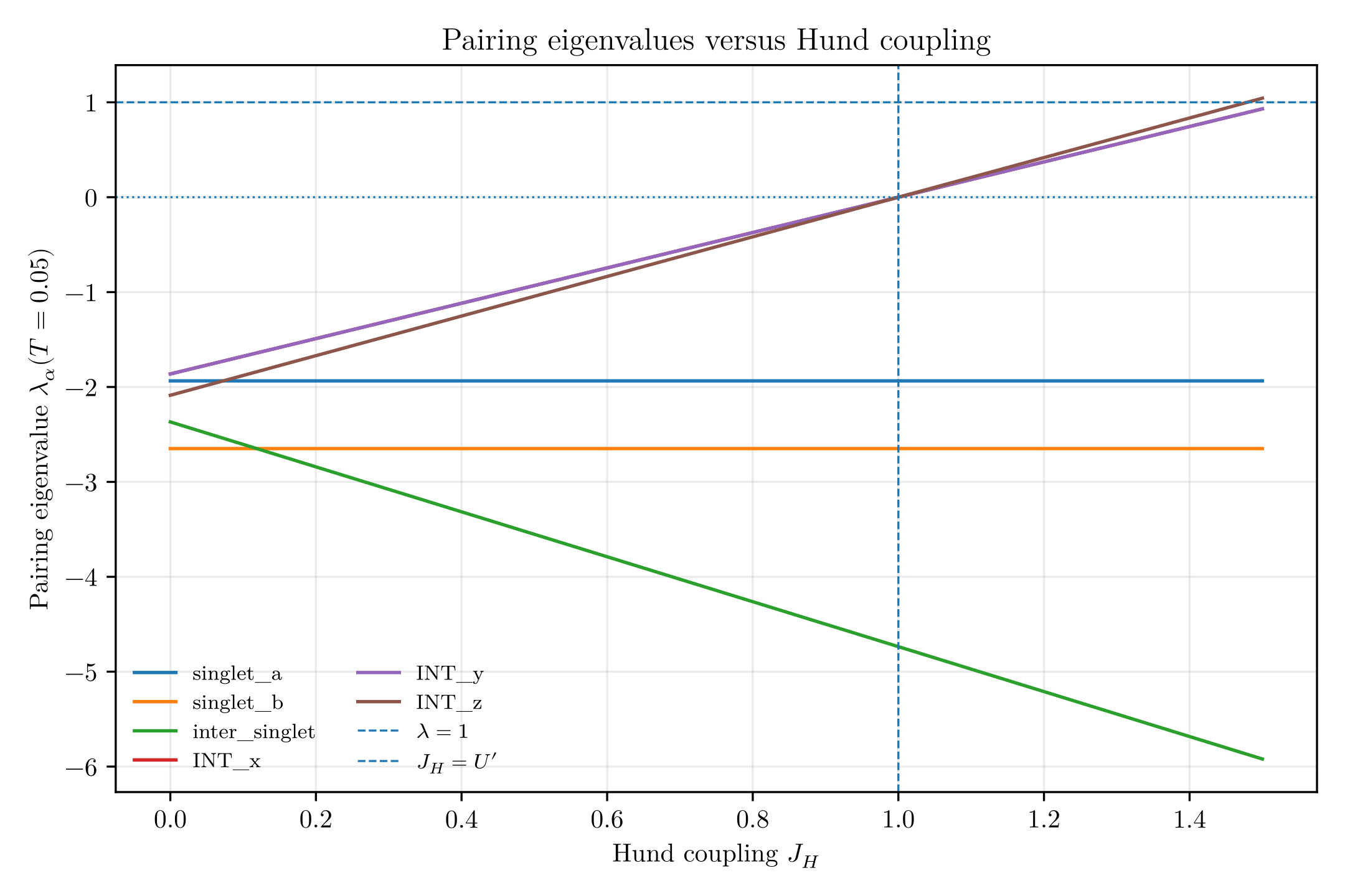
Figure 8.17: Linearized local-channel diagnostic. The plotted eigenvalues are (\lambda_\alpha=-\mathbf U_\alpha\chi_\alpha), equivalently the scalar inverse-susceptibility kernel (\mathcal K_\alpha=\chi_\alpha^{-1}+\mathbf U_\alpha) crossing zero at (\lambda_\alpha=1). Hund exchange raises the internally antisymmetric equal-spin triplet sector relative to interorbital singlet competitors, but the conservative bare hierarchy remains repulsive unless (J_H>U’) or an effective attractive INT vertex is supplied.
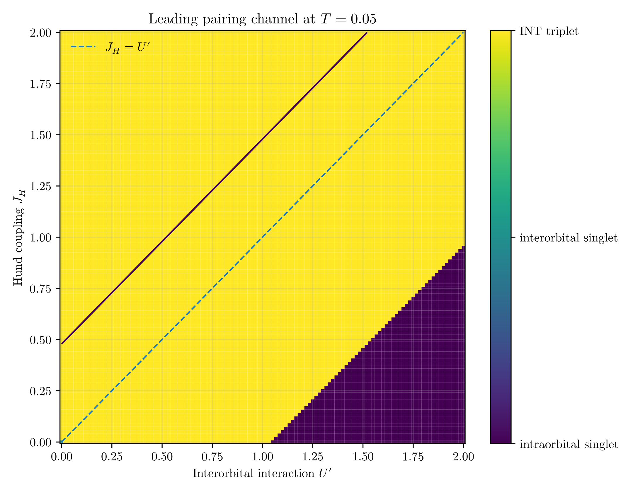
Figure 8.18: Leading local channel map. The map records the leading channel label, not a nonlinear self-consistent ground state.
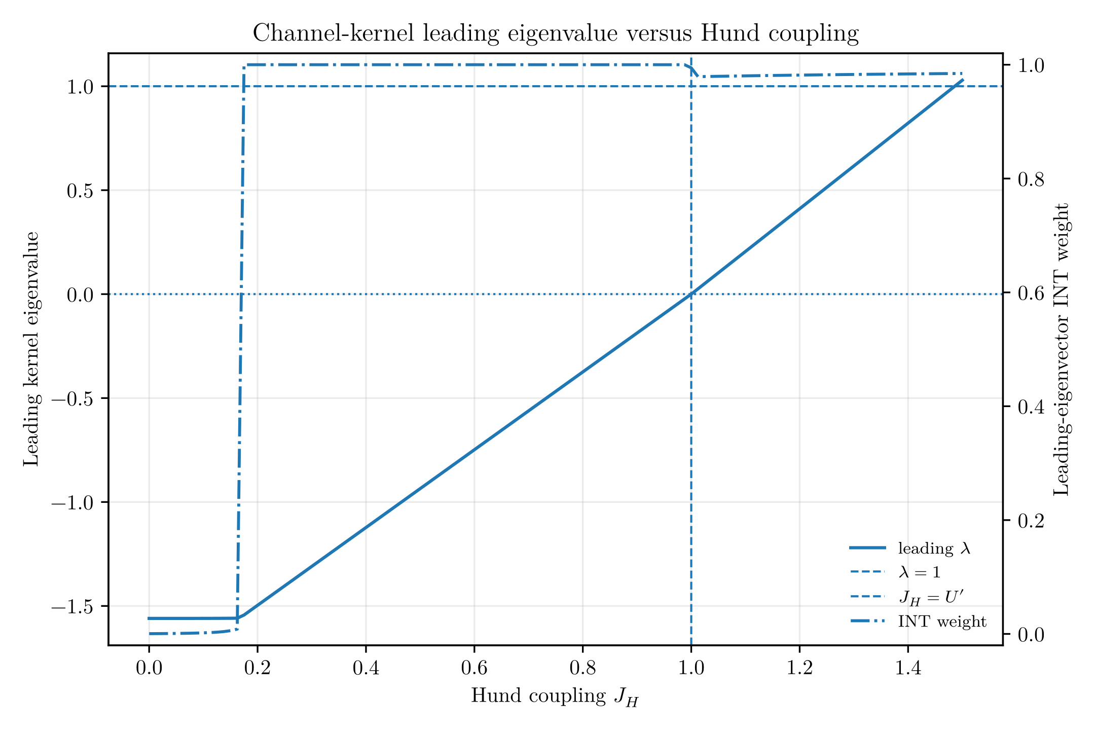
Figure 8.19: Projected coupled-kernel scan versus Hund exchange.
The local INT gap is even in momentum and spin triplet, so the antisymmetry required by Fermi statistics resides in the orbital labels. In the internal basis ((a\uparrow,a\downarrow,b\uparrow,b\downarrow)),
Equivalently,
The minus signs in the matrix are the entries of the antisymmetric orbital tensor (i\tau_y). The state is nonunitary when
in the paired subspace, equivalently (i\mathbf d\times\mathbf d^*\ne0) [25]. Unequal equal-spin amplitudes, (|\Delta_{\uparrow\uparrow}|\ne|\Delta_{\downarrow\downarrow}|), split the nonzero eigenvalues of (\Delta\Delta^\dagger). This algebraic split is the diagnostic used below.
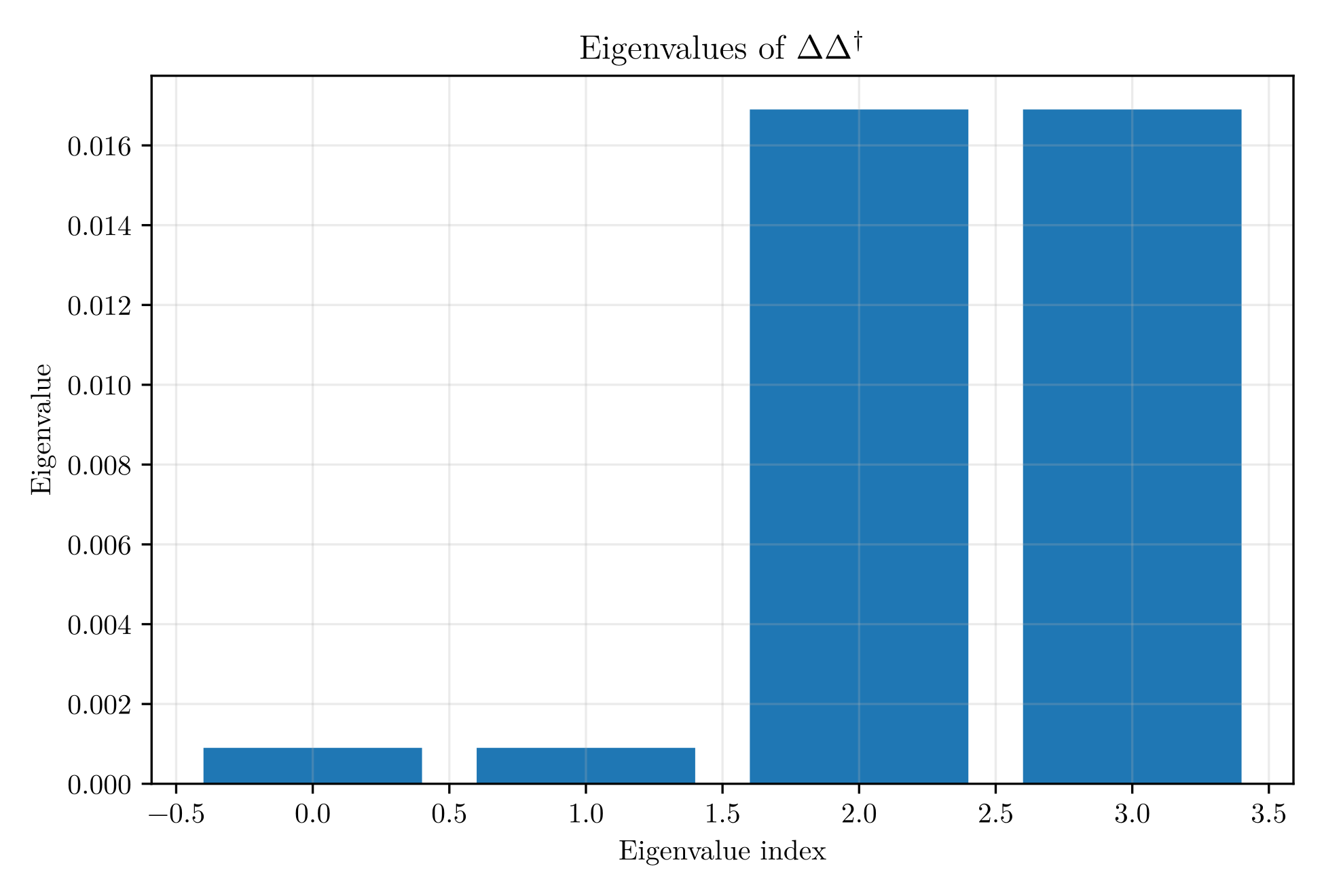
Figure 8.20: Eigenvalues of (\Delta\Delta^\dagger) for the imposed nonunitary INT gap. Unequal equal-spin components split the eigenvalues, showing that (\Delta\Delta^\dagger) is not proportional to the identity in the paired subspace.
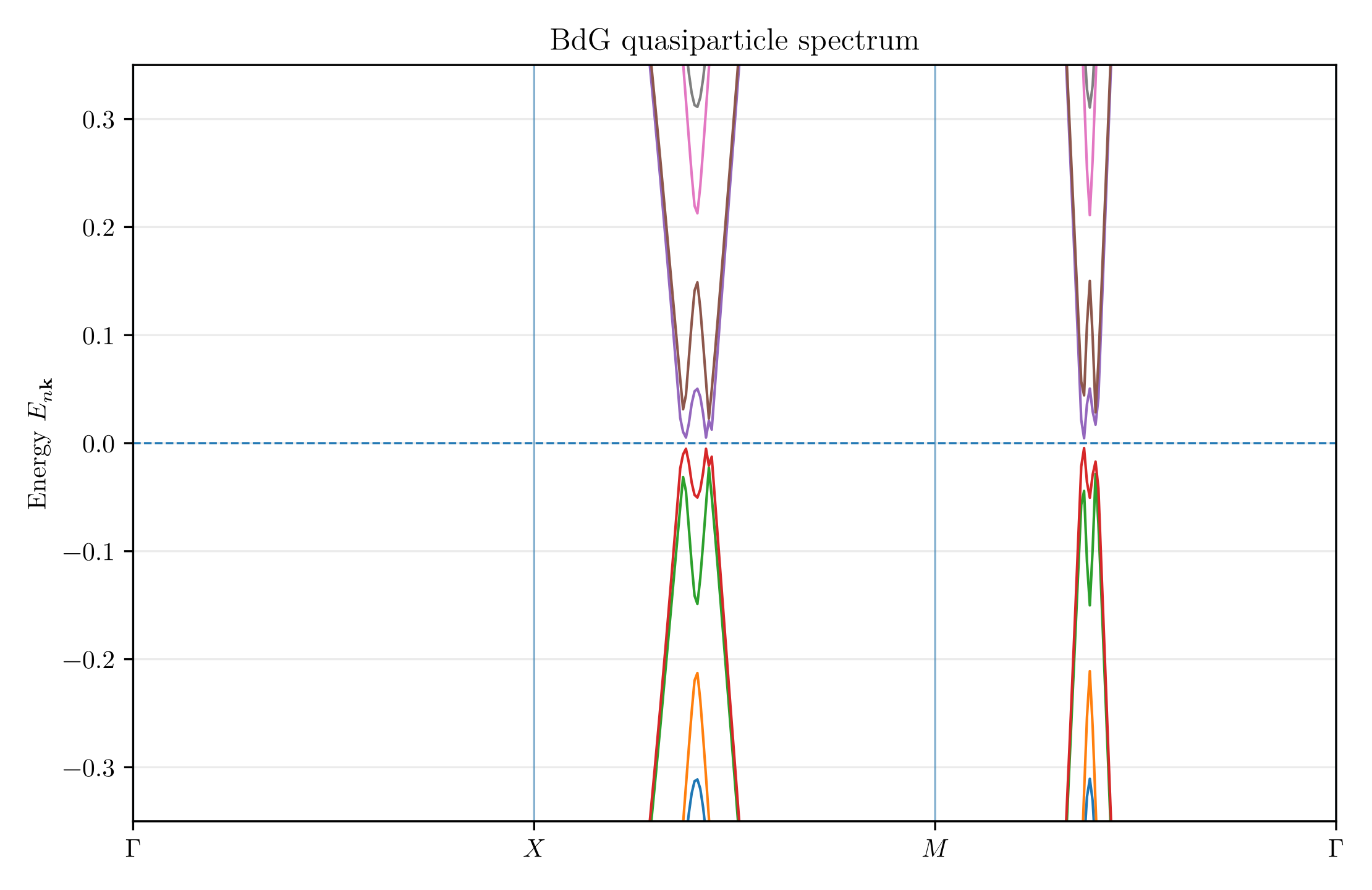
Figure 8.21: BdG quasiparticle spectrum for the imposed INT state.
The spin-resolved density of states is computed from the electron block of the retarded BdG Green function,
where (\Pi_s) projects onto spin (s=\uparrow,\downarrow), and (\eta) is the Lorentzian broadening. Before the impurity/Dyson step this is the spectral sum
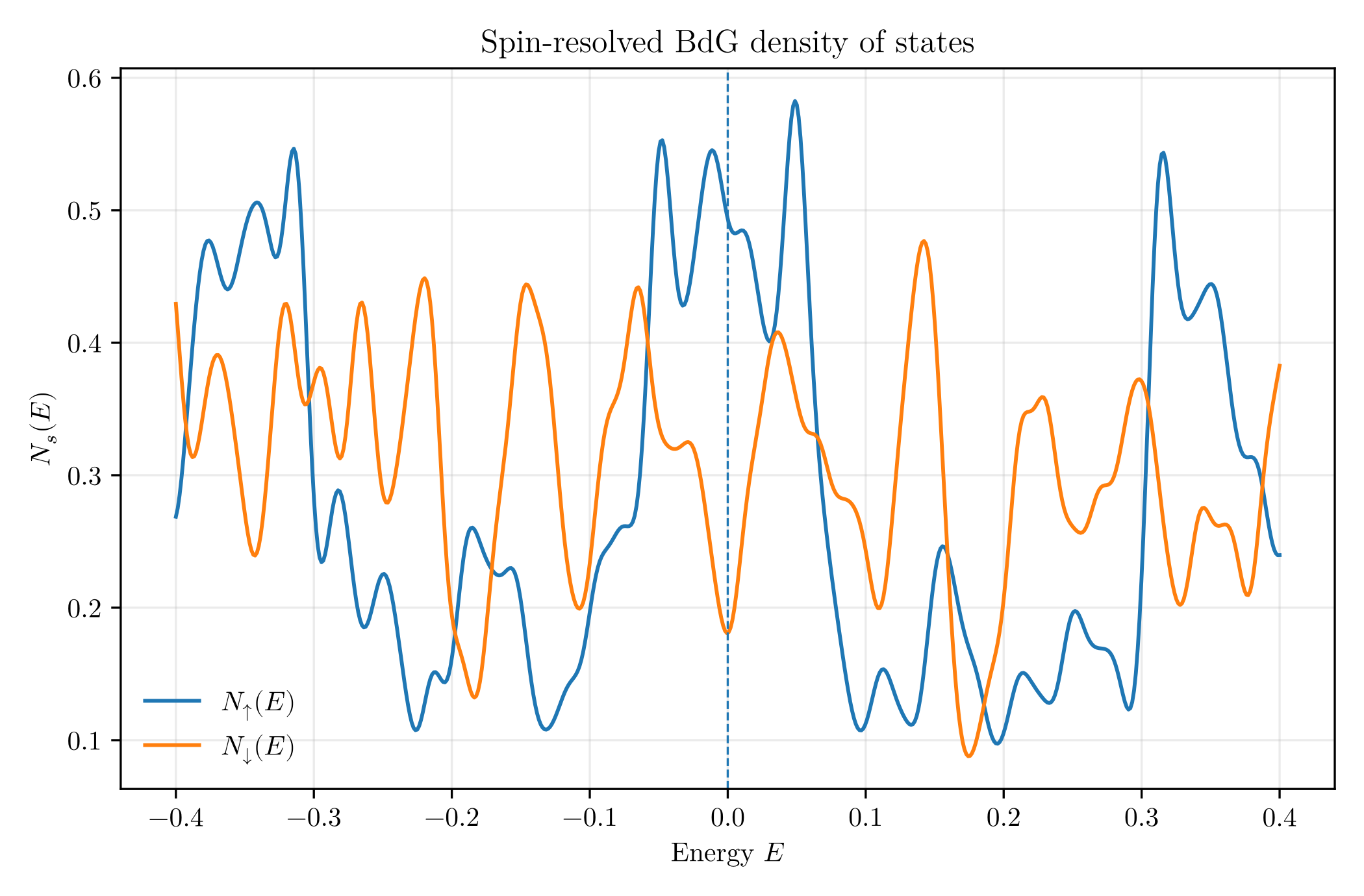
Figure 8.22: Spin-resolved density of states for the imposed INT ansatz. The nonunitary gap produces spin-resolved spectral asymmetry, but this imposed diagnostic does not by itself prove self-consistent phase selection.
Channel selection is not enough. The weak-pairing gap is the local INT matrix projected into the Fermi subspace,
A large local gap is ineffective if it maps a Fermi-level state mainly to a partner outside the retained low-energy subspace. This obstruction is clear in the representative Hamiltonian
Here (\xi(\mathbf k)) is a scalar dispersion, (\tau_y) is the orbital-antisymmetric hybridization/SOC structure, and the (\lambda_x\sigma_x,\lambda_z\sigma_z) terms are spin-orbital texture components. In this convention, (\lambda_z\sigma_z) is longitudinal with respect to the equal-spin quantization axis, while (\lambda_x\sigma_x) is transverse. This terminology is basis dependent.
The helicity projectors are
Using the equal-spin convention
the (\Delta_x) used in the projection rule denotes
For the simplified Hamiltonian above, the nonzero singular values of (P_\nu\Delta_{\rm INT}P_\nu^T) scale as
A purely longitudinal texture therefore leaves the same-helicity INT projection zero in this limit. A transverse spin-orbital component repairs the weak-pairing projection by rotating the normal-state eigenvectors so that the INT-paired partner stays in the low-energy subspace.
The plotted projection diagnostics are evaluated on
with
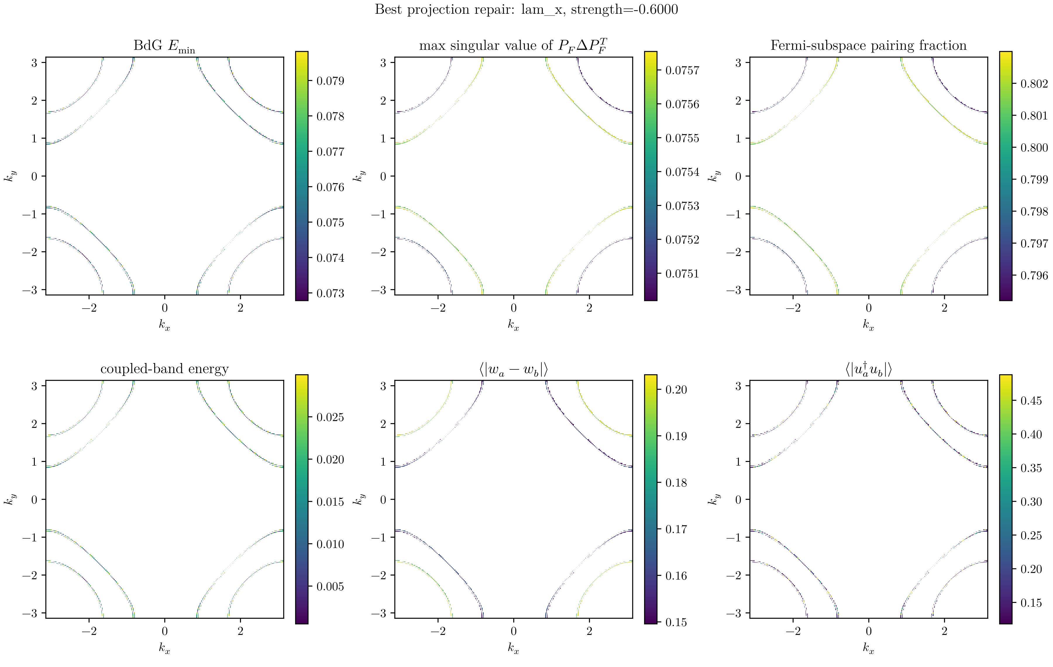
Figure 8.23: Fermi-subspace projection repair. The weak-pairing gap is controlled by (\Delta_F(\mathbf k)=P_F(\mathbf k)\Delta_{\rm INT}P_F^T(-\mathbf k)), not by the local INT matrix alone. In the minimal toy model the INT operator mostly pairs a Fermi-level state with a partner outside the retained low-energy subspace. A transverse spin-orbital texture repairs this by keeping the INT-paired partners in the same Fermi subspace; increasing scalar attraction alone does not solve the projection problem.
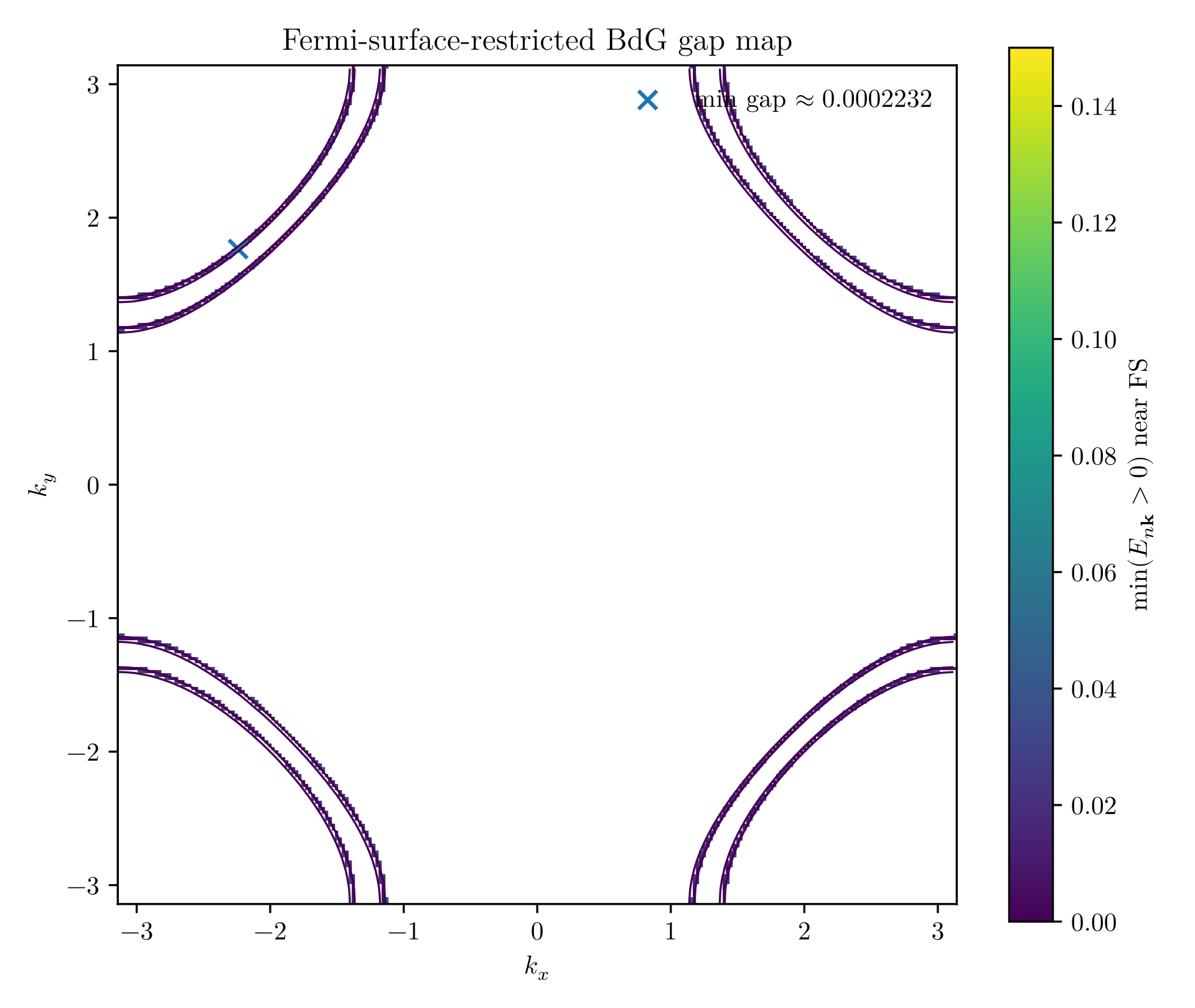
Figure 8.24: Fermi-surface gap map for the toy INT state.
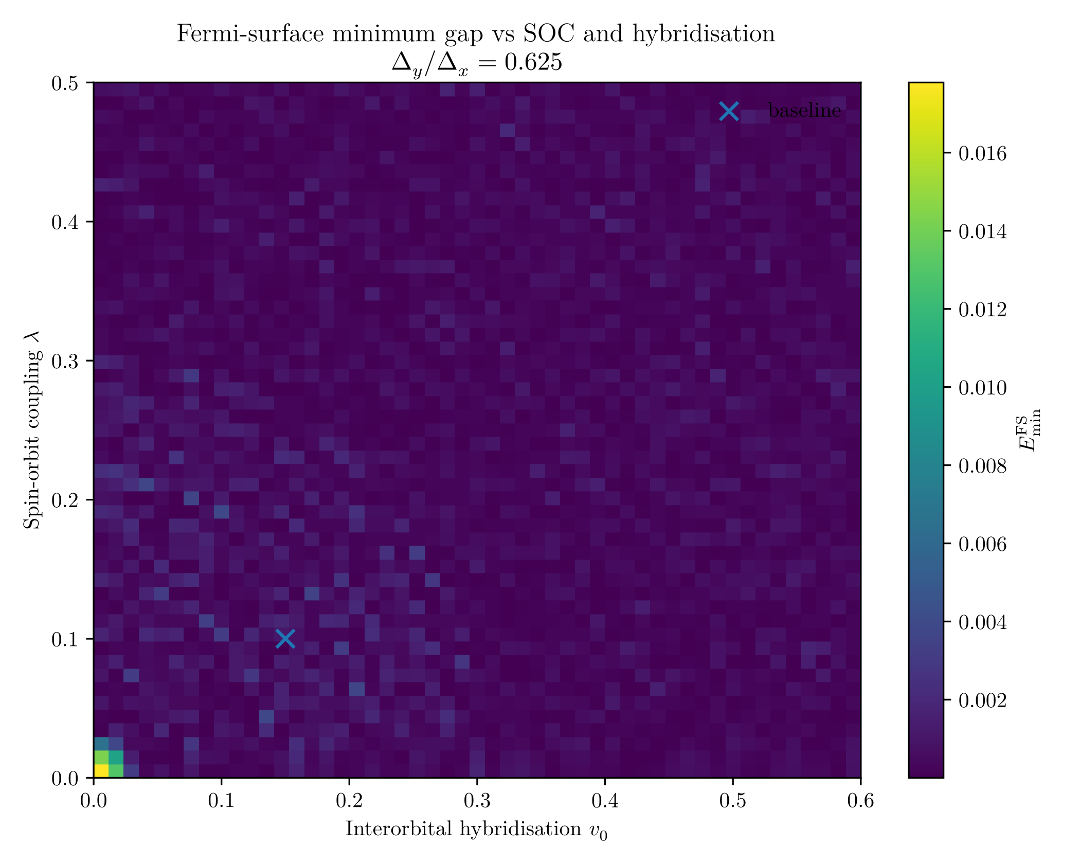
Figure 8.25: Minimum gap scan versus spin-orbit hybridisation.
The BdG Hamiltonian used in the self-consistent tests is
For a local antisymmetrized interaction tensor (\mathbf U),
with (\ell) combining orbital and spin. The normal density and anomalous Gor’kov contraction are
The mean-field decoupling is
with self-consistency fields
An anomalous-only update keeps only (\Delta[\chi]). A density-density Hartree update keeps the diagonal direct pieces of (\phi[\rho]). The compact unrestricted Kanamori feedback keeps local Hartree/Fock normal contractions together with the anomalous update. The compact tests are reduced-basis benchmarks; the first full-basis material scans remain quick anomalous-first calculations, not production full-Wannier unrestricted Hartree-Fock-Gor’kov minimizations.
The ranked thermodynamic quantity is
where the constants remove the particle-particle and particle-hole double counting introduced by the decoupling. At finite temperature,
up to the common normal-state reference used in branch comparisons.
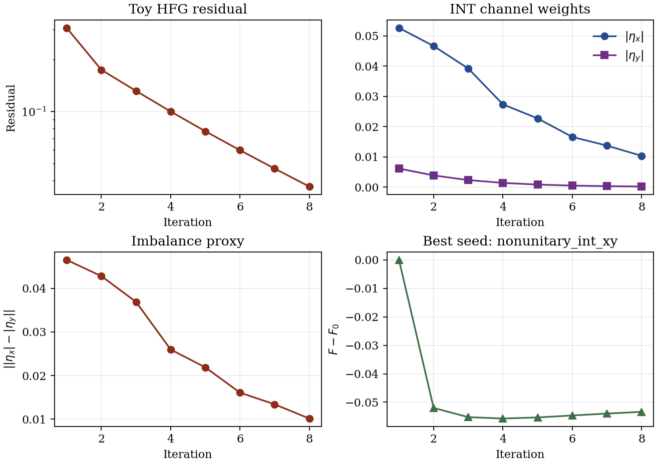
Figure 8.26: Representative toy HFG convergence trace. The residual, INT channel weights, imbalance proxy, and free-energy change converge in the same calculation used for the phase-selection benchmark. Convergence alone does not imply nonunitary phase selection; in this run the imbalance proxy remains small compared with the relaxed pairing scale.
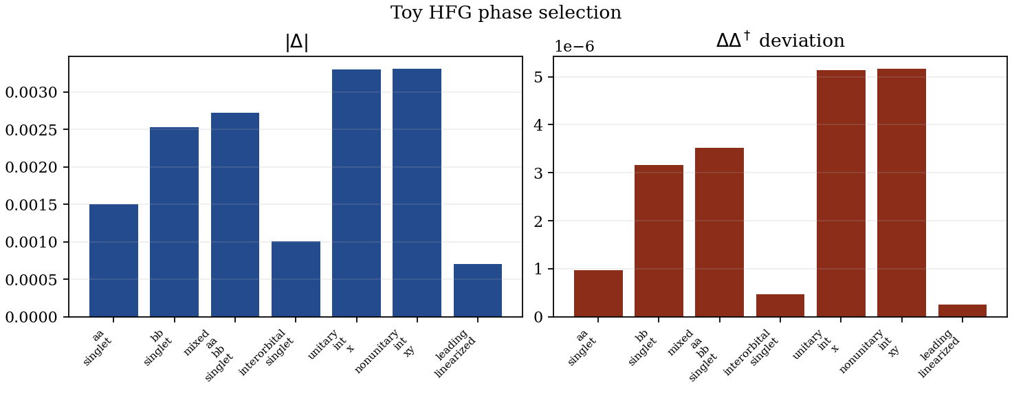
Figure 8.27: Toy Hartree-Fock-Gor’kov phase selection. The constrained nonunitary branch is a diagnostic ansatz, while free relaxation favors a unitary or competing branch unless additional spin-polarization feedback is supplied.
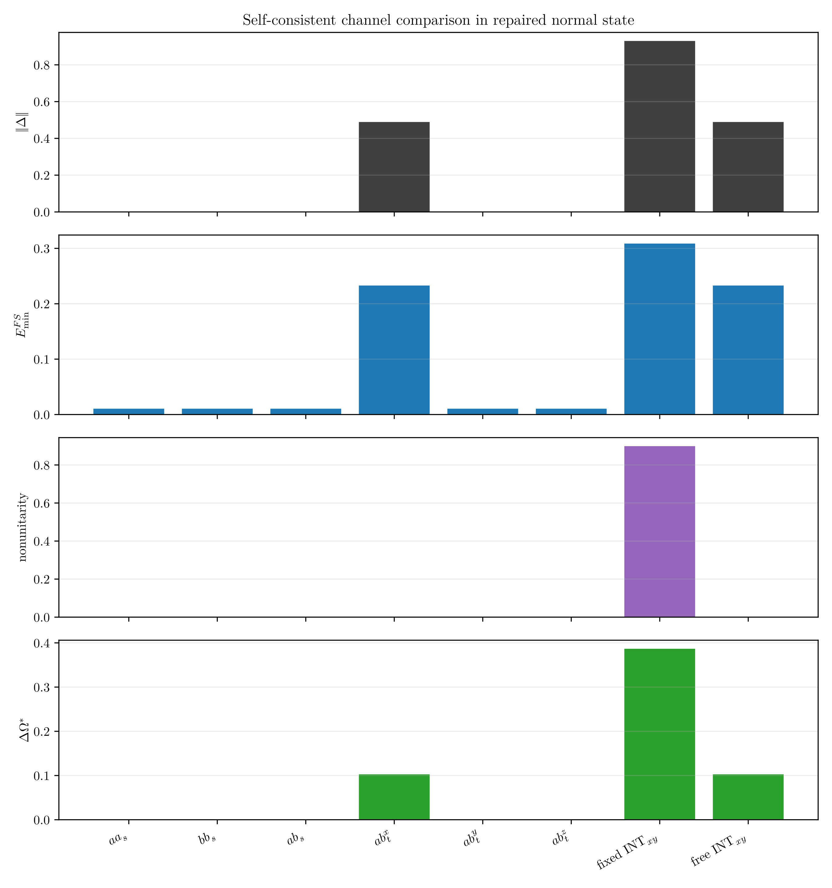
Figure 8.28: Self-consistent channel comparison.
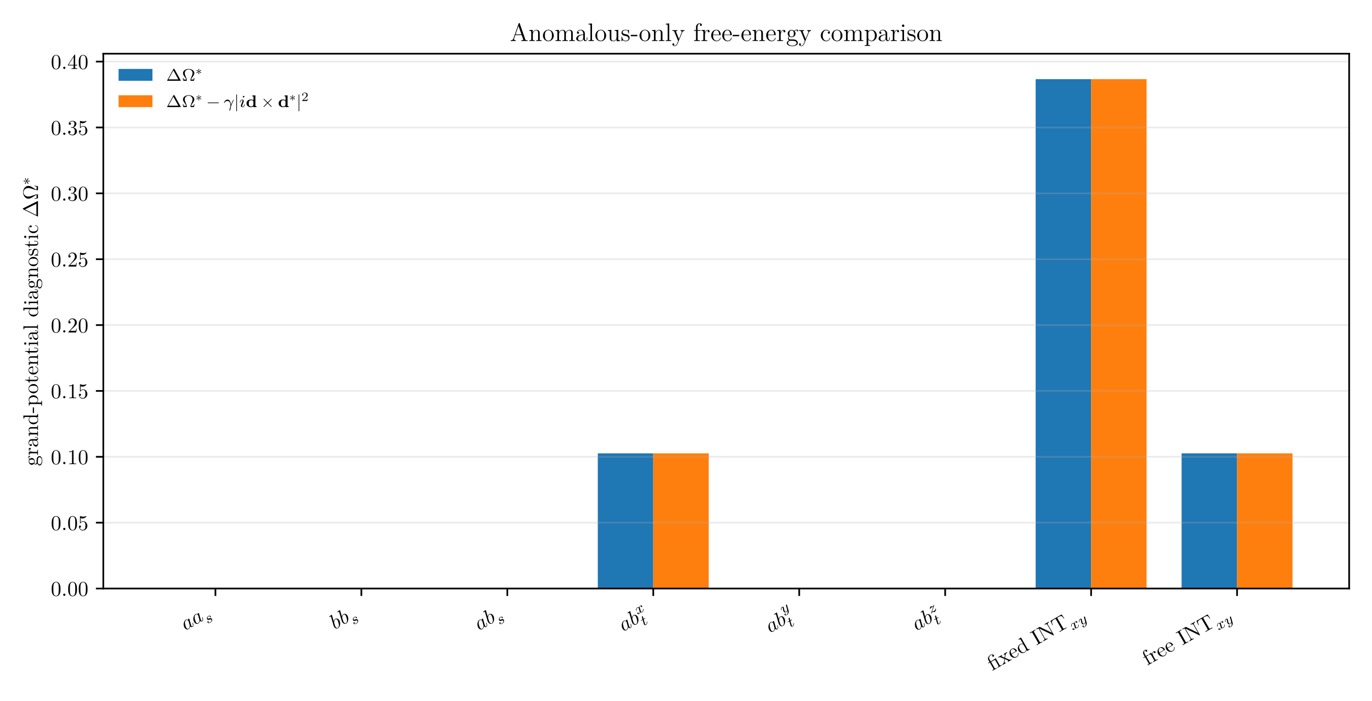
Figure 8.29: Self-consistent free-energy comparison.
The calculations separate scalar pairing attraction from nonunitary imbalance selection. A scalar attractive INT vertex controls the total triplet amplitude. It does not automatically favor (|\Delta_{\uparrow\uparrow}|\ne|\Delta_{\downarrow\downarrow}|). A minimal phenomenological route to stabilize nonunitarity would be a normal spin-polarization feedback term, for example
Both (\mathbf M) and (i\mathbf d\times\mathbf d^*) are odd under time reversal, so this coupling does not impose an external magnetic field. Minimizing over (\mathbf M) gives
leaving the two time-reversed domains to be chosen spontaneously. The present material calculations do not include such a tuned channel unless it is generated by the Kanamori feedback being tested.
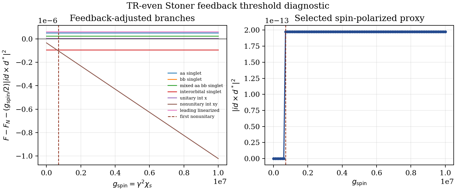
Figure 8.30: Reduced Stoner-feedback threshold diagnostic. A finite feedback strength is required before the spin-polarized nonunitary seed becomes the lowest branch in this reduced landscape.
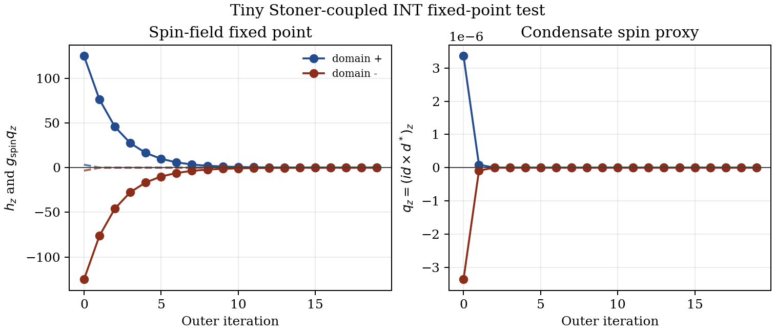
Figure 8.31: Tiny Stoner-coupled INT fixed-point test. The two time-reversed nonunitary seeds start with opposite normal spin fields and condensate spin proxies, but the coupled loop relaxes back toward zero field and zero (i\mathbf d\times\mathbf d^*) for the tested toy parameters.
The Stoner comparison is an implementation benchmark, not an additional material claim. It follows the density-channel functional used in Whittlesea’s thesis [31],
The ordinary density Stoner benchmark magnetizes with the expected sign convention, while the particular INT condensate-coupled loop still relaxes to zero for the tested toy parameters.
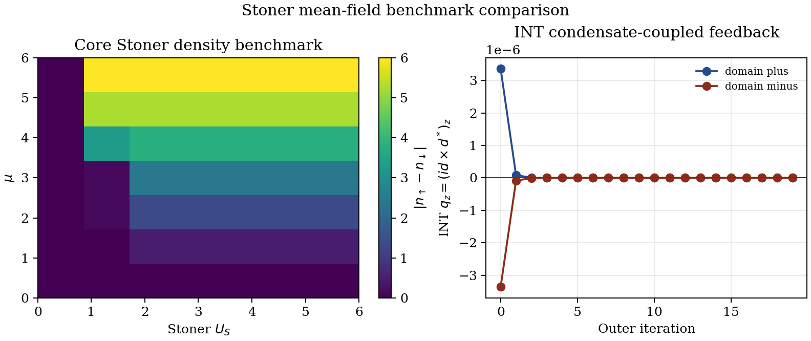
Figure 8.32: Stoner mean-field benchmark comparison. Left: density-channel Stoner benchmark following Whittlesea’s thesis, obtained by minimizing (F_{\rm Stoner}); the magnetic region in the ((U_S,\mu)) plane confirms the implemented sign convention. Right: INT condensate-coupled feedback; the condensate spin proxy relaxes to zero for the tested toy parameters.
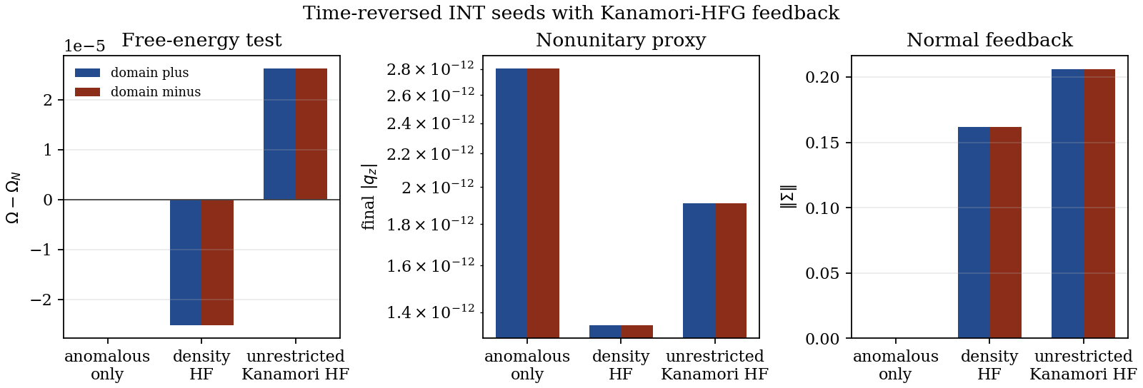
Figure 8.33: Time-reversed INT seeds with compact Kanamori-HFG feedback. The anomalous-only, density-density Hartree/Fock, and unrestricted Kanamori Hartree/Fock updates are run from two nonunitary seeds related by time reversal. The density and unrestricted feedback modes generate finite normal fields, but the final (q_z=(i\mathbf d\times\mathbf d^*)_z) remains at numerical floor for the tested tiny parameters.
The material-derived survey applies the same diagnostics to spin-orbit-coupled LaNiC(_2) and LaNiGa(_2) Wannier Hamiltonians. The workflow is Quantum ESPRESSO SCF, Quantum ESPRESSO NSCF on the Wannier mesh, pw2wannier90, Wannier90, import of wannier90_hr.dat, a shift to the QE Fermi reference, and then reduced- and full-basis INT diagnostics. The spin-orbit runs use noncollinear QE inputs with noncolin=.true. and lspinorb=.true.; the retained input files use ecutwfc=80, ecutrho=640, Marzari-Vanderbilt smearing, and degauss=0.02.
| Input | SCF/NSCF mesh | (N_b/N_W) | final spread |
|---|---|---|---|
| LaNiC(_2) SOC | (8^2\times6 / 6^2\times4) | (320/88) | (206.16,{\rm A}^2) |
| LaNiGa(_2) SOC | (6^2\times4 / 6^2\times4) | (360/176) | (929.75,{\rm A}^2) |
| LaNiC(_2) SOC dense | (10^2\times8 / 8^2\times6) | (320/88) | (285.54,{\rm A}^2) |
The active dense LaNiGa(_2) SOC Hamiltonian came from Icarus job 9011002. A later staged full-path smoke check, Icarus job 9011065, completed and generated the overlay below. It gives a near-(E_F) RMSE of (0.475,{\rm eV}) and the QE run reported two unconverged eigenvalues at one k point. This is provenance for a survey Hamiltonian, not production-quality validation.
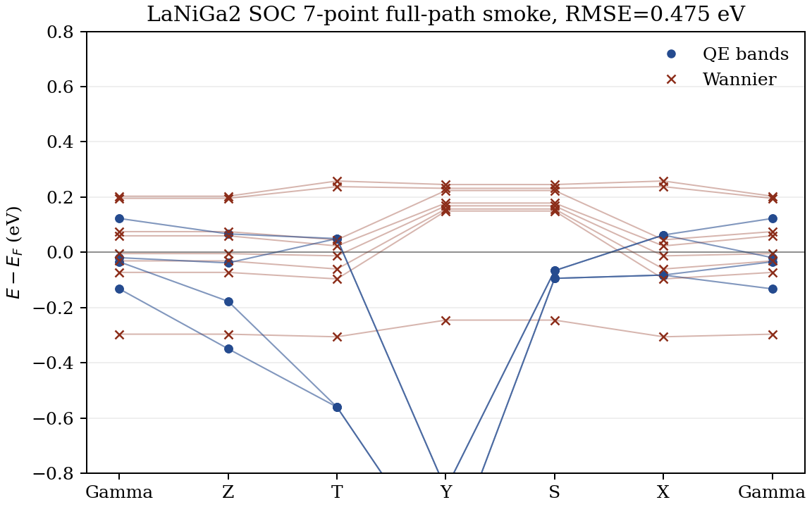
Figure 8.34: LaNiGa(_2) SOC Wannier partial overlay smoke check. QE-direct bands and the Wannier interpolation are overlaid on the staged seven-point high-symmetry-path calculation near (E_F). The comparison is useful provenance, but the mismatch and QE warning mean this is not a full Wannier validation.
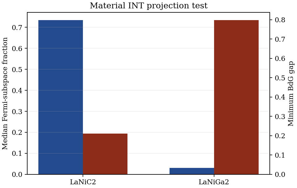
Figure 8.35: Reduced material INT projection. The active dense LaNiGa(_2) SOC reduction has weak INT Fermi-subspace projection in the current four-state truncation, and projection alone does not determine the relaxed phase.
| Material | (R) | (P_{\rm INT}) | best seed | (\Omega_{\rm MF}-\Omega_N) | (q) |
|---|---|---|---|---|---|
| LaNiC(_2) SOC | 245 | 0.735 | unitary INT | (4.68\times10^{-6}) | (1.16\times10^{-6}) |
| LaNiGa(_2) SOC | 245 | 0.031 | unitary INT | (1.37\times10^{-5}) | (2.14\times10^{-6}) |
Here (R) is the number of retained Wannier real-space translation blocks, (P_{\rm INT}) is the median retained INT Fermi-subspace projection, and (q) is the scalar-identity deviation of (\Delta\Delta^\dagger). Values (q\sim10^{-6}) are numerical-noise scale in these scans.
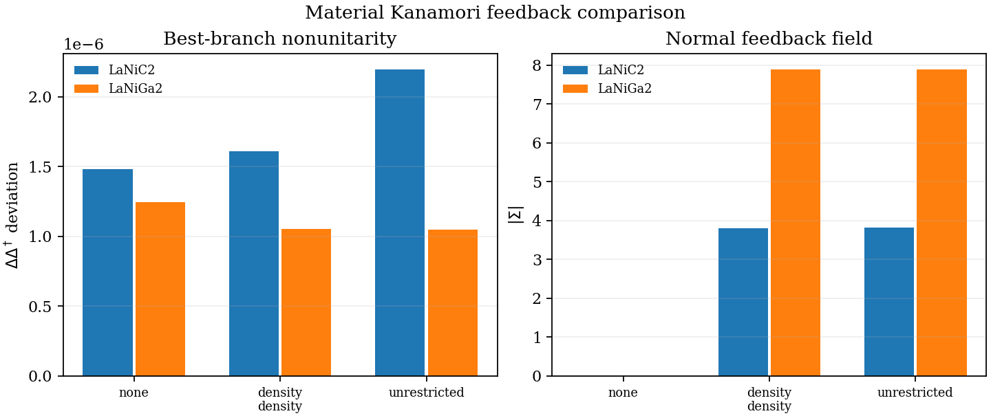
Figure 8.36: Kanamori feedback comparison in the reduced material basis. Including normal-field feedback changes the compact free-energy landscape but does not stabilize a robust nonunitary INT branch.
The full-basis quick scan removes the four-state truncation but remains anomalous-first. Both active materials select onsite singlet rather than INT in this first scan, remain above the normal reference in the quick free-energy estimate, and have best nonunitarity at numerical-noise scale.
| Material | active dimension (N) | best seed | (\Omega_{\rm MF}-\Omega_N) | (q) |
|---|---|---|---|---|
| LaNiC(_2) SOC | 88 | onsite singlet | (5.76\times10^{-5}) | (9.45\times10^{-7}) |
| LaNiGa(_2) SOC | 176 | onsite singlet | (5.54\times10^{-6}) | (8.99\times10^{-8}) |
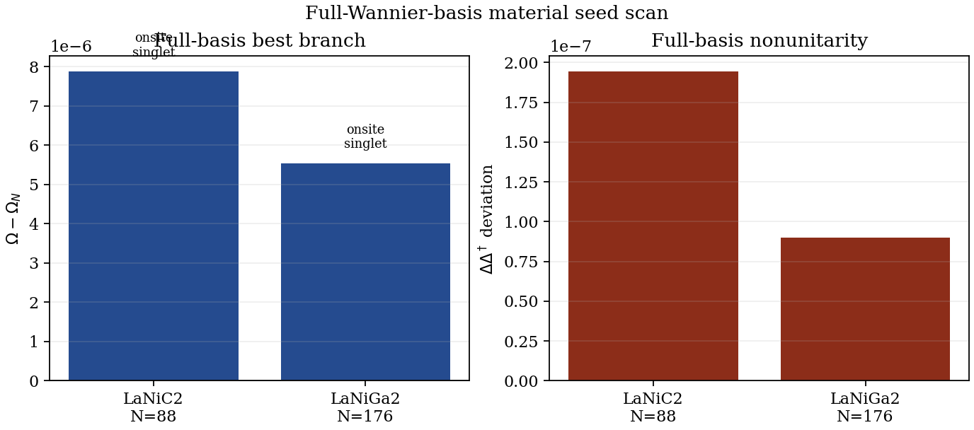
Figure 8.37: Full-basis material seed scan. Keeping the full active Wannier basis removes the reduced four-state truncation and gives onsite-singlet-like winners for both LaNiC(_2) and LaNiGa(_2) SOC survey Hamiltonians.
The code reserves (\mathbf U) for the bare local Kanamori interaction tensor. In self-consistency scans, the bare tensor (\mathbf U=(U,U’,J_H,J_P)) is distinct from the attractive vertex used in a normalized anomalous channel. Legacy figure parameters still quote the positive effective channel magnitude as (g_{\rm pair}); in this chapter it should be read as (|U^{\rm eff}{\rm INT}|), not as the bare repulsive (V{\rm INT}=U’-J_H).
The retained two-orbital toy normal state uses (t=1), (\mu=-2.7), (s=0.1), (v_0=0.15), (v_1=0), and baseline longitudinal spin-orbit coupling (\lambda_z=0.1). The displayed repaired toy example turns on (\lambda_x=0.6). The toy HFG convergence uses (|U^{\rm eff}{\rm INT}|=2.8), (U=3.0), (J_H=0.6), temperature (T=0.03), a (3\times3) mesh, mixing (\gamma=0.35), and 8 iterations. The reduced material figures use (|U^{\rm eff}{\rm INT}|=1.6), a (3.0,{\rm eV}) Fermi window, a (5\times5) projection grid, and a (2\times2) HFB mesh for 5 iterations. The feedback comparison uses (U=3.0), (J_H=0.6), a (3\times3) HFB mesh, (\gamma=0.3), and tolerance (10^{-7}). The first full-basis scan uses (|U^{\rm eff}_{\rm INT}|=1.2), a (1\times1) HFB mesh, (\gamma=0.35), and tolerance (10^{-6}).
For material-derived calculations, the normal-state hoppings are read from Wannier90 real-space Hamiltonian files. All material Hamiltonians are shifted so that the chosen QE Fermi reference is zero; the quick scans therefore use (\mu=0) after this shift and do not impose an additional fixed-filling constraint.
The retained figures are generated from the QuLab INT module, qulab.research.int. The main regeneration command in the publication source is:
1python -m qulab.research.int.scripts.generate_figuresAdding --include-retained-scans regenerates the older scan inventory. The material inputs live under the QuLab lanix2_wannier data directory. The active survey Hamiltonians are the LaNiC(_2) Zhang-2018 SOC and LaNiGa(_2) full SOC wannier90_hr.dat files, with QE/Wannier provenance in the colocated manifest.json, scf.in, nscf.in, wannier90.template.json, and wannier90.wout files. The curated PRB manuscript archive for this thesis chapter is stored in publication/; the canonical paper source remains ~/Workspaces/henry/publications/int-self-consistency-prb at commit 1ca438f.
The material Hamiltonians are survey Wannier models with large spreads, not production-quality interpolations. This is especially important for LaNiGa(_2): the staged overlay is a smoke check, not a validated full-path interpolation near (E_F). The full interaction feedback is also incomplete at production scale. The compact tests include unrestricted Kanamori feedback, but the full-basis scans are quick anomalous-first calculations rather than production full-Wannier unrestricted Hartree-Fock-Gor’kov minimizations.
The completed evidence is a local-channel diagnostic, imposed BdG algebraic and spectral diagnostics, toy and compact HFG feedback tests, Stoner sign-convention benchmarking, and quick reduced/full-basis material surveys. What remains missing for a strong material claim is a production-quality SOC Wannier basis, a clean full-path DFT/Wannier overlay near (E_F), explicit filling or chemical-potential control beyond the QE Fermi shift, a full-basis unrestricted HFG feedback calculation, and robustness against interaction, seed, mesh, and Wannier-window choices.
INT pairing remains a coherent constrained channel and a useful diagnostic ansatz. It naturally connects Hund-favored interorbital triplet pairing, even-parity orbital antisymmetry, split (\Delta\Delta^\dagger), spin-resolved spectra, and condensate spin-polarization diagnostics. The self-consistency tests are the restrictive step. Scalar INT attraction does not by itself select a nonunitary imbalance, and the current material-derived LaNiC(_2)/LaNiGa(_2) survey Hamiltonians relax to unitary or onsite-singlet-like branches with nonunitarity at numerical-noise scale.
The defensible conclusion is therefore negative at survey level: the present local Hubbard-Kanamori-like calculations validate the INT ansatz as a channel and observable diagnostic, but they do not derive it as a robust self-consistent material ground state.
Having met the Meissner Effect in our previous chapter, that is, the total expulsion of magnetic fields inside superconductors, it may surprise the reader to discover there is an entire class of unconventional superconductors exhibiting intrinsic magnetic fields, spectacularly contradicting the Meissner Effect. Magnetism in materials have diverse microscopic origins, and time-reversal symmetry breaking (TRSB) superconductors are no exception, with different classes of them requiring different theories. These theories have a sense of momentum, which is a logical route to TRSB, because one need only have a system in which the electrons (or electron pairs, rather) circulate in one way, rather than the other, a classical picture of motion. This thesis is built around a more intrinsically quantum mechanical notation of time-reversal symmetry breaking, based on the orientation of the complex phase of the macroscopic superconducting state, called a Loop Supercurrent [22]; we also explore another route to TRSB through a multiorbital spin-triplet theory, which is known to exist in other materials.
Mathematically, time reversal is denoted by and is understood to be antiunitary, which means it is not a linear operator (one cannot achieve time-reversal (TR) in a continuous manner, it is intrinsically discontinuous). When a system is mathematically symmetric in time, we refer to it as time-reversal symmetric (TRS), and when such a system’s solutions break the TRS, we refer to such states as TRSB.
The standard textbook route to TRSB in a superconductor is a chiral momentum-space state such as or , usually described as a two-component order parameter selected from a two-dimensional irreducible representation. That route will be retained here because it is the canonical reference case. It is not, however, the primary organising principle of this thesis.
A central claim of the thesis is that TRSB need not be understood primarily through momentum-space chiral pairing states such as . Instead, TRSB can arise through internal winding of a multicomponent superconducting order parameter, with the broken-symmetry state selected by microscopic free-energy minimisation. The loop-supercurrent framework of Ghosh, Annett, and Quintanilla provides the main theoretical starting point for this alternative route. [22, 32]
This distinction is forced by the material motivation. LaNiC and LaNiGa both show TRSB signatures, yet the usual 2D-irrep route is not naturally available in their orthorhombic setting. The relevant multicomponent structure must therefore be internal, arising from spin, orbitals, bands, or symmetry-related sites within a unit cell. The chapter is organised around that problem.
The discussion proceeds from symmetry criteria to free-energy mechanisms. Conventional chiral states are introduced first as a contrast class. The emphasis then shifts to multicomponent GL theory, frustration, internal phase winding, and unit-cell loop supercurrents, with LaNiC and LaNiGa providing the main materials motivation throughout.
Figure 8.38: Schematic overview of superconducting routes relevant to the present chapter. The conventional -wave state and the established unconventional reference cases of -wave and -wave pairing are included to orient the discussion in familiar terms. The loop-supercurrent mechanism is the new route developed in this thesis: TRSB is carried by internally structured multicomponent order parameters whose relative phases wind within a unit cell and break time-reversal symmetry without relying on a natural two-dimensional crystal irrep.
Figure 8.39: Timeline of reported TRSB superconductors, shown by discovery year and superconducting transition temperature (T_c), with colors/symbols indicating material class. In most materials, the microscopic mechanism underlying TRSB remains debated; only the earliest heavy-fermion examples, ((\mathrm{U,Th})\mathrm{Be}_{13}) and (\mathrm{UPt}_3), are longstanding canonical multicomponent candidates, whereas even (\mathrm{Sr_2RuO_4}) remains under active debate. [33, 34, 35]
Two materials recur throughout this thesis because they provide a natural paired case in the TRSB literature. TRSB has been reported in both LaNiC and LaNiGa, but LaNiC is noncentrosymmetric whereas LaNiGa is centrosymmetric. This makes it difficult to explain both materials using only the standard noncentrosymmetric parity-mixing narrative without introducing additional internal structure. [36, 27, 37, 32]
In both materials the principal experimental signature is the same: in zero applied field, ZF-SR detects an additional relaxation or field distribution that appears at, or just below, , consistent with spontaneous internal fields generated by the superconducting state. [26, 27, 32]
At the same time, thermodynamic probes often look comparatively conventional. In LaNiGa, several analyses favour a fully gapped, two-gap-like superconducting state. In LaNiC, the extent of gap anisotropy or nodal structure remains more sample- and probe-dependent, and recent work argues for two-gap TRSB superconductivity in the same material family. [28, 29, 32]
That LaNiGa line of argument is especially useful here because it makes the tension explicit: TRSB points toward a nonunitary triplet interpretation, while thermodynamic data look fully gapped rather than nodal. The 2016 preprint version of the two-gap LaNiGa analysis, together with Quintanilla’s short research blog note, is a concise entry point to that puzzle and to the proposed same-spin, different-orbital pairing resolution. [28, 38]
More recently, normal-state NMR, NQR, magnetization, XPS, and DFT measurements on LaNiGa have argued against strong magnetic fluctuations or strong Stoner enhancement in the normal state. That does not by itself determine the superconducting order, but it does sharpen the motivation for mechanisms in which TRSB is selected by internal multicomponent structure rather than by a strongly correlated magnetic normal state. [39]
The LaNiC/LaNiGa pair is also not isolated. Recent SR and thermodynamic work on the noncentrosymmetric 111 family LaNiSi, LaPtSi, and LaPtGe reports the same broad combination of ingredients: a fully gapped superconducting state together with spontaneous TRSB at . In that case the normal state is argued to be a Weyl nodal-line semimetal, so the onset of TRSB superconductivity is expected to drive a topological transition as well. That broadens the significance of the present thesis: internal multicomponent TRSB is not only a puzzle for two orthorhombic intermetallics, but part of a wider material landscape where unconventional superconductivity coexists with nontrivial normal-state band topology. [40]
The crystallographic contrast between the pair is already informative. LaNiC crystallises in the orthorhombic noncentrosymmetric Amm2 setting, whereas LaNiGa crystallises in the orthorhombic centrosymmetric Cmmm setting with three inequivalent Ga sites. The structural figures below are included for one reason only: to make that internal contrast visible before the later electronic-structure discussion. [41, 42, 43]
LaNiC2 overview

LaNiC2 local motif

Native QTT views of the reported LaNiC crystal structure. The overview emphasises the noncentrosymmetric La-Ni-C chain network, while the local view highlights the short C motif together with its neighbouring Ni and La environment. The thesis-facing point is simply that a reduced Ni/C internal description is structurally plausible for later effective descendants. [41, 44]
LaNiGa2 overview

LaNiGa2 local coordination

Native QTT views of the reported LaNiGa crystal structure. The overview and local motif make clear that the low-energy problem is multiorbital and internally structured even before superconductivity is introduced. But unlike LaNiC, the thesis does not treat local coordination as the decisive materials input here; the later normal-state symmetry and Wannier discussion must carry that burden. [45, 43]
The structural point of these figures is therefore modest. Local coordination pictures can make the unit cell legible, but they do not determine the superconducting mechanism. For LaNiC they suggest that an internal Ni/C reduction may be meaningful; for LaNiGa they mainly warn that the problem is too multiorbital and symmetry-constrained to be read off from a neighbour graph. The physics burden therefore passes quickly from structure to electronic structure: projected bands, spin-orbit splitting, Wannier reduction, and the symmetry of the low-energy manifold. [46, 44, 47]
It is also useful to separate the existing microscopic literature on this material pair into three layers. First, there are conventional first-principles electronic-structure and electron-phonon studies, such as the Subedi-Singh calculation for LaNiC, Zhang et al.’s DFT and de Haas–van Alphen simulation paper for LaNiC, Singh’s fermiology study of LaNiGa, and the later DFPT analysis of LaNiGa by Tütüncü and Srivastava. Second, there are DFT-informed superconductivity papers that solve a semiphenomenological BdG- or KKR-based model on top of the ab initio electronic structure. Third, there are the later symmetry- and topology-focused papers, especially for LaNiGa, which establish the nonsymmorphic Dirac-line / Dirac-loop normal-state setting that any serious low-energy theory must preserve. [48, 49, 50, 51, 30, 47]
Within the literature surveyed for this thesis, no standard parameter-free superconducting density-functional calculation in the Oliveira-Gross-Kohn sense was identified for either LaNiC or LaNiGa. The nearest published microscopic results instead sit on the DFT-informed BdG side. That distinction matters for the later modelling chapters, because it means the existing literature already points toward a materials-faithful multiorbital BdG programme, but not yet to a settled ab initio SCDFT explanation of the pairing interaction.
For LaNiC, the clearest example is the 2018 paper by Csire, Újfalussy, and Annett, who describe a first-principles-based semiphenomenological Dirac-BdG treatment of nonunitary triplet pairing. Their central thermodynamic comparison is reproduced below. The thesis-facing point is not merely that a nonunitary triplet state can be written down, but that the nodal candidate is disfavoured while fully gapped interorbital equal-spin states remain viable. In their fit, the pairing strengths are fixed by requiring the self-consistent calculation to reproduce the experimental , so the paper remains DFT-informed BdG rather than parameter-free SCDFT. [52]
Figure 8.40: Literature figure reproduced from Csire, Újfalussy, and Annett [52], cropped from their Fig. 7. The nodal - equal-spin state fails at low temperature, while the fully gapped - and - interorbital equal-spin states both track the measured specific heat much more closely.
For LaNiGa, the closest existing quantitative superconductivity paper is the 2020 work of Ghosh, Annett, Gradhand, and Quintanilla. It starts from ab initio electronic structure and magnetic information, then introduces a phenomenological interorbital equal-spin pairing interaction on the Ni sector. The paper again uses a single adjustable interaction, fixed by the experimental , and the supplementary material explicitly formulates the technical implementation in KKR / Kohn-Sham-Dirac-BdG language. The figure reproduced below is therefore especially useful for this thesis: it ties together three quantities that any later microscopic model should try to reproduce simultaneously, namely the specific heat, the spontaneous internal moment below , and the two-gap spin-resolved quasiparticle density of states. [30, 53]
Figure 8.41: Literature figure reproduced from Ghosh, Annett, Gradhand, and Quintanilla [30], cropped from their Fig. 3. The calculation simultaneously reproduces the specific heat, the onset of a spontaneous magnetic moment below , and a two-gap spin-resolved quasiparticle DOS for an interorbital equal-spin pairing state between Ni and orbitals.
Taken together, these papers set the immediate target for the later modelling chapters. They do not yet provide a standard SCDFT account of superconductivity in LaNiC or LaNiGa, but they do show that DFT-informed multiorbital BdG theory can already reach experimentally meaningful observables. The next step for the present thesis is therefore not to start from a neighbour graph or a hand-drawn bond model, but to build symmetry-faithful low-energy models that can test whether the observed TRSB is better understood through nonunitary interorbital pairing, internally winding orbital order, or a combination of both. For LaNiGa, that programme must in particular remain compatible with the later nonsymmorphic normal-state literature, where the low-energy Dirac-line / Dirac-loop structure constrains the admissible superconducting models from the outset. [47, 39]
These materials therefore motivate two broad microscopic routes:
The thesis focus is the second route. The reason is not that the first route is excluded, but that LaNiC and LaNiGa demand a framework in which TRSB can emerge from internal multicomponent structure even when the familiar chiral-momentum-space explanation is not naturally enforced.
That is the narrative handoff to the later materials chapter. The background task is to explain why LaNiC and LaNiGa force the problem beyond the standard two-dimensional-irrep story. The materials task is then narrower and harder: determine what symmetry-faithful low-energy basis and what candidate pairing structures remain viable once the actual normal-state electronic structure is respected.
| Material | Inversion | Symmetry setting | (typ.) | Main TRSB evidence | Gap phenomenology | Thesis-facing significance |
|---|---|---|---|---|---|---|
| LaNiC | absent | orthorhombic, noncentrosymmetric | ZF-SR onset of spontaneous internal fields at or near | broadly conventional thermodynamics; nodal or anisotropic structure debated | motivates TRSB without a natural 2D-irrep explanation | |
| LaNiGa | present | orthorhombic, centrosymmetric | ZF-SR onset of spontaneous internal fields at or near | often described as fully gapped with two-gap phenomenology | shows that the mechanism cannot be reduced to noncentrosymmetric parity mixing |
Terminology. “Two-component TRSB” here means a (nearly) degenerate two-component order parameter (often a 2D irrep) whose relative phase is complex, e.g. . [25] This is not the same as “multiorbital spin-triplet”, where internal orbital/band structure supplies the relevant multicomponent degree of freedom even if the crystal irrep is 1D. [32] “Nonunitary triplet” is a distinct TRSB route: can occur already for 1D irreps, with TRSB residing in internal spin structure rather than a chiral basis function. [27, 37] “Two-gap superconductivity” is spectral phenomenology: it means two distinct gap scales are inferred from low-energy quasiparticles (often associated with different Fermi-surface sheets) and does not, by itself, specify singlet vs triplet, unitary vs nonunitary, or orbital-diagonal vs interorbital pairing. In LaNiGa a prominent proposal is precisely that an interorbital equal-spin, nonunitary triplet state produces a fully gapped two-gap spectrum [28], but the reverse implication is not generally valid: two-gap behaviour can also occur in multiband singlet superconductors, including TRSB multiband singlet states such as [54]. A multiband example where the broken-symmetry state is often described as rather than a symmetry-protected 2D-irrep chiral state is BaKFeAs. [54] This is why LaNiC/LaNiGa are not clean textbook 2D-irrep chiral examples: the likely multicomponent structure is internal (spin/orbitals/bands) within an orthorhombic setting. [32, 28]
The mechanism classes used in this thesis are summarised in Table 2.1. Standard chiral momentum-space states are included mainly as a reference class against which the internally winding mechanisms of interest are contrasted.
| Mechanism class | Source of multicomponent structure | TRSB variable | Typical field phenomenology | Role in this thesis |
|---|---|---|---|---|
| Chiral state from 2D irrep | crystal symmetry, two-dimensional irrep | relative phase , e.g. | often edge-, defect-, or domain-wall-dominated | standard reference case, not the main mechanism here |
| Nonunitary triplet | internal spin structure, often with SOC | local and strongly screened spontaneous fields | major alternative mechanism for LaNiC/LaNiGa | |
| Unit-cell loop supercurrents | inequivalent sites or orbitals within a unit cell | internal phase winding and loop chirality | intra-cell currents; fields concentrated near disorder and domains | central microscopic mechanism of the thesis |
| Complex mixing of two 1D channels | near-degenerate pairing channels | relative phase between two scalar order parameters | weak bulk fields with strong domain dependence | useful bridge beyond the 2D-irrep route |
| Multiband or multi-orbital frustration | three or more coupled internal phases | phase structure | defect- and domain-wall-dominated fields | generic precursor to internally winding TRSB states |
A superconducting order parameter is not merely a scalar gap amplitude. In a weak-coupling description the gap matrix transforms under the symmetry group of the normal state, and the allowed superconducting states are classified by irreducible representations of the crystal point group. In GL language, the order-parameter components are coordinates in the irrep space. Standard symmetry-based treatments are given in [25].
For a one-dimensional irrep, the primary order parameter is usually a single complex scalar. For a multidimensional irrep, several complex components condense and relative phases become physical low-energy degrees of freedom. This is the usual symmetry route to TRSB at the superconducting transition.
That route is important as a reference point, but it is not sufficient for the present thesis. In LaNiC and LaNiGa, the relevant orthorhombic point groups do not provide the natural two-dimensional irrep structure that would make the standard chiral explanation automatic. The multicomponent degree of freedom must instead be internal.
Time reversal is antiunitary. It complex-conjugates amplitudes and reverses momenta and spins. A superconducting state preserves TRS only if the order parameter is invariant under up to global gauge redundancy and, when relevant, up to basis changes inside a degenerate internal subspace.
This is the key point used repeatedly later: every superconductor is described by a complex order parameter, but TRSB does not mean merely that the order parameter is complex. It means that the complex structure cannot be removed by gauge choice.
At the many-body or mean-field level, a superconducting state preserves TRS if there exists a global phase such that
TRSB means that no such exists.
At the level of the pairing kernel, for spin- electrons with unitary spin part ,
must hold for some global phase . Failure of this condition is a practical TRSB criterion.
At the Bogoliubov–de Gennes (BdG) level, TRS means the existence of an antiunitary operator such that
Experimentally, TRSB is inferred through observables odd under , such as spontaneous internal fields, Kerr rotation, or anomalous interference.
A practical consequence is that spontaneous TRSB produces a discrete degeneracy: if is a TRSB state, then is distinct and degenerate in zero field. Domain formation is therefore generic, and weak-field probes are often dominated by domain walls, disorder, or boundaries rather than by a uniform bulk moment.
For a multicomponent order parameter , the GL free energy has the schematic form
where the terms encode the allowed symmetry couplings between components. Minimisation determines whether the ordered state preserves or breaks TRS.
For a two-component order parameter transforming as a two-dimensional irrep, a standard quartic free-energy density is
Write
and define the relative phase
If , the minimum is typically realised by a real configuration and TRS is preserved. If , minimisation favours
which is realised by
These states break TRS because time reversal maps to and the two are not gauge-equivalent.
This is the standard textbook route to chiral momentum-space states such as or . It is included here as the reference case, but it is not the primary organising principle for the material systems studied in this thesis.
TRSB does not require a multidimensional crystal irrep. It can also arise when two distinct one-dimensional pairing channels are nearly degenerate. Let and be complex scalar order parameters associated with two one-dimensional irreducible representations. The quartic coupling
locks the relative phase through .
If , the minimum occurs at or and the coexistence state preserves TRS. If , the minimum occurs at
so the coexistence state takes the form and breaks TRS.
This mechanism is already closer to the thesis viewpoint, because the decisive issue is not momentum-space chirality by itself but free-energy selection among multiple internal order-parameter components.
Later chapters work with explicit mean-field and BdG Hamiltonians. The phase-locking terms that appear in GL theory arise microscopically by introducing multiple pairing fields, integrating out the fermions, and expanding the resulting effective action in powers of those fields:
When amplitudes are relatively stiff, the long-wavelength reduction is a phase theory,
with generated by intercomponent pair scattering.
This phase-only form is the natural bridge to internally winding TRSB states. The relevant components need not correspond to distinct Fermi pockets. They can be orbitals or inequivalent sites inside one unit cell. Once that happens, phase frustration becomes an internal free-energy problem rather than a momentum-space chirality problem.
TRSB frequently appears as the resolution of phase frustration. Several couplings try to lock relative phases to incompatible values, and the system lowers its free energy by choosing intermediate phase differences that are neither nor . The resulting complex structure is physical and cannot be removed by a global gauge transformation.
This mechanism is important for two reasons. First, it gives a general route to TRSB in multiband and multi-orbital superconductors without requiring a chiral spatial basis function. Second, it maps directly onto loop-supercurrent constructions in which the relevant phases live within a single unit cell.
In a minimal description one introduces
and writes
For there is no frustration: the single preferred phase difference can always be satisfied. For , competing signs and magnitudes of the couplings can produce incompatible constraints.
The canonical frustrated pattern is
together with its time-reversed partner
The order-parameter manifold then has a structure: the usual overall superconducting phase and a discrete chirality selecting one of two time-reversed minima.
The components need not label different bands. In a Wannier or orbital basis they can label inequivalent internal degrees of freedom within one unit cell. Pair-hopping terms again reduce to phase-locking terms between the corresponding phases.
If the internal coupling graph contains loops, the minimal case being a triangle, frustrated couplings can stabilise circulating bond supercurrents,
Two opposite circulation patterns are then related by time reversal and define a loop chirality. This is the microscopic content of the internal-winding mechanism used later in the thesis.
A frustration-driven TRSB state forms domains in zero field because the two time-reversed minima are degenerate. Domain walls support spatial variation of the relative phases and can carry supercurrents and local magnetic fields even when the uniform bulk magnetisation is negligible.
This is why TRSB signatures are often experimentally subtle. The symmetry breaking is robust, but the observable fields may be concentrated near defects, disorder, or domain boundaries and further reduced by Meissner screening. [55, 56]
TRSB is inferred through responses that are odd under time reversal. No single experiment measures the order parameter directly.
ZF-SR detects changes in the local magnetic-field distribution below through enhanced muon-spin depolarisation or relaxation. It is highly sensitive to small internal fields and is therefore central to the LaNiC/LaNiGa discussion. Its interpretation nevertheless requires care: SR detects local fields, not order-parameter phase directly, and the measured signal can be dominated by domain structure or inhomogeneous field localisation. [57, 58, 32]


Polar Kerr rotation probes TRS-breaking optical response and therefore complements SR. Phase-sensitive Josephson interferometry probes superconducting phase structure more directly. Scanning SQUID or Hall imaging constrains whether spontaneous fields are edge-like, defect-bound, or associated with domain walls. These distinctions matter because internally winding and loop-current states are naturally expected to produce highly nonuniform local fields. [59, 60, 61, 62]
The key symmetry constraint is simple. In many canonical TRSB superconductors, including the usual chiral reference cases, TRSB at the primary transition is naturally explained by a multidimensional irrep: two order-parameter components condense together and a relative phase such as is selected. In LaNiC and LaNiGa, the relevant orthorhombic point groups have only one-dimensional irreducible representations, so the simplest chiral-irrep mechanism is not naturally available.
The two materials nevertheless differ in a way that matters for the later SOC discussion. LaNiC is noncentrosymmetric with point group (C_{2v}) (mm2), so antisymmetric spin-orbit coupling and parity mixing are symmetry-allowed ingredients of a material Hamiltonian. LaNiGa is centrosymmetric with point group (D_{2h}) (mmm), so it does not reduce to the same antisymmetric-SOC story even though it shares the orthorhombic one-dimensional-irrep constraint. This is why the thesis treats spin-orbit texture as a material-specific projection problem rather than as a generic SOC/no-SOC switch.
This is why these materials are central here. They force the multicomponent structure to be internal rather than inherited directly from crystal representation theory. Historical reference systems such as SrRuO or UPt remain useful contrasts, but they are not the organising centre of the present thesis. [63, 59, 64, 60]
A GL mechanism emphasised in this material family is that a superconducting instability in a triplet channel can couple linearly to a subdominant magnetisation and thereby lower the free energy of a nonunitary TRSB state. [27, 30, 32]
Within the LaNiGa discussion, the crucial microscopic claim is not merely that the state is triplet, but that pairing can occur between electrons of the same spin on different orbitals. That preserves overall fermionic antisymmetry while allowing an even-parity, fully gapped, two-gap superconducting state that still breaks time-reversal symmetry. This was the central interpretation advanced in the 2016 LaNiGa penetration-depth / heat-capacity / upper-critical-field analysis and highlighted in the accompanying commentary. [28, 38]
A useful earlier notebook calculation makes the practical ambiguity of this proposal concrete. In a two-orbital impurity model, the spin-resolved local spectrum distinguishes the multiorbital-singlet and nonunitary-triplet cases rather clearly at low broadening, but the total local DOS becomes much harder to tell apart once the phenomenological broadening is increased to the scale of the orbital splitting. That is precisely why the earlier notebook work treated QPI and other structured probes as more discriminating than a broadened tunnelling spectrum by itself.
Author calculation from the earlier two-orbital impurity-model notebook. Left: the low-broadening case (\epsilon=0.0125) resolves the spin/orbital structure cleanly. Right: at (\epsilon=0.1) the same spin-resolved spectra are visibly smeared, although the nonunitary-triplet branch still retains an internal asymmetry between the spin channels. The model uses (43\times 43) sites, an impurity at the origin with (V/t=1.21), and the original parameter sets used in the earlier notebook comparison.
Figure 8.42: Author calculation from the same two-orbital impurity-model notebook. Left: at low broadening (\epsilon=0.0125), the multiorbital-singlet and nonunitary-triplet spectra can still be separated in the total local DOS. Right: at larger broadening (\epsilon=0.1), the two become much less distinguishable. The comparison uses (43\times 43) sites, (\mu=0), rigid orbital splitting (s/t=0.05), interorbital hybridisation (\delta/t=0.075), pairing scale (\Delta/t=1), interorbital shift (\varsigma/t=0.35), and an impurity at the origin with (V/t=1.21), sampled at (\mathbf r=[5,0]).
The newer normal-state study is useful here as a counterweight. If LaNiGa lacks strong precursor magnetic fluctuations in the normal state, then any successful TRSB mechanism has to work without leaning too heavily on the usual strongly correlated narrative. That makes internally structured order parameters, multiorbital pairing, and unit-cell-scale phase structure even more relevant to the thesis viewpoint. [39]
The 111-family result is useful for a different reason. There the argument is not built around LaNiGa-style same-spin different-orbital pairing, but around a minimal spin-triplet description of superconductivity emerging from a Weyl nodal-line normal state. That provides a second route by which TRSB, full gaps, and nontrivial normal-state topology can coexist, and it is therefore an important wider backdrop for the thesis emphasis on internal superconducting structure beyond the simplest chiral-irrep story. [40]
For a spin-triplet superconductor the order parameter may be encoded by a complex vector. In a reduced GL description one may use a complex vector order parameter . A standard TRSB diagnostic is the nonunitarity vector
If , the state is unitary. If , the state is nonunitary and breaks TRS.
Importantly, can be nonzero even when the crystal irrep is one-dimensional. The TRSB then resides in the internal spin structure of the condensate rather than in a chiral momentum-space basis function.
Introduce a subdominant magnetisation and write
with .
If is subdominant, minimisation at quadratic order gives
Substituting back yields
The negative sign is the key result. Any configuration with nonzero is favoured by this coupling. A nonunitary TRSB state can therefore be stabilised already at even though the crystal point group has only one-dimensional irreducible representations. [27, 37, 28, 30]
For illustration, take
Then
so the state is nonunitary, TRSB, and induces .
The loop-supercurrent framework is the culmination of the present chapter. Its central claim is that TRSB can be selected by free-energy minimisation in an internal Josephson network formed by superconducting phases attached to inequivalent sites or orbitals within one unit cell. The broken symmetry is then carried by internal phase winding rather than by a conventional momentum-space chiral basis function.
This is the route that most directly matches the thesis. It naturally produces small, local spontaneous fields, it accommodates orthorhombic materials in which a 2D-irrep explanation is not available, and it makes the relevant degree of freedom a loop chirality rather than a macroscopic edge-current pattern. [22, 32]
Suppose several superconducting components associated with inequivalent internal degrees of freedom are coupled in a frustrated way. The unit cell then acts as an internal Josephson network. If the coupling graph contains loops and the preferred phase differences are incompatible, the minimum is a compromise phase pattern with circulating bond supercurrents.
The two opposite circulation patterns are related by time reversal and form a pair. TRSB is therefore tied to a discrete choice of loop chirality. This is the internally winding alternative to standard chiral momentum-space pairing.
On a lattice or network the gauge-invariant phase difference on a bond is
The corresponding bond current is proportional to . Summing link phases around a closed path gives a loop holonomy. In the present setting that holonomy is not a formal gauge-theory detour; it is the natural collective coordinate for internally frustrated superconducting phases on a fixed microscopic network.
The effective two-component order parameter relevant for loop supercurrents is not a two-component crystal-irrep order parameter. It arises instead from a doubly degenerate superconducting instability at quadratic order in a subspace spanned by two time-reversed loop-current basis states and . [22]
Expand
so that the order parameter is
Time reversal exchanges the basis states and implies
Write
and define the relative phase
The quartic free energy in this instability subspace reduces to
with
Minimising over the amplitude gives
For , so that , the ground state is found by minimising .
The minima occur in time-reversed pairs:
which exchange and and therefore correspond to opposite loop-supercurrent circulation. In a special regime there is a continuous ring of degenerate minima satisfying
The relevant structural point is that the effective two-component space here is internal. It is generated microscopically from orbitals, sites, or bands and then resolved by quartic free-energy minimisation into a pair of internally winding TRSB states.
This chapter has established the main conceptual framework used throughout the thesis for discussing TRSB in superconductors. Standard chiral momentum-space pairing from a two-dimensional irrep remains the canonical textbook route to TRSB, but it serves here mainly as a contrast class. The central emphasis is that TRSB can also arise from internal multicomponent structure, with the broken-symmetry state selected by microscopic free-energy minimisation. When phase locking among internal superconducting components is frustrated, the resulting state acquires a structure, forms domains, and generates weak but symmetry-diagnostic spontaneous fields.
LaNiC and LaNiGa are important because they motivate TRSB mechanisms that are not naturally explained by the standard 2D-irrep route. Within this material family, nonunitary triplet order coupled to a subdominant magnetisation provides one symmetry-consistent mechanism. The central thesis mechanism, however, is that loop supercurrents can carry TRSB through internal phase winding and a discrete loop chirality inside the unit cell.
Later chapters construct microscopic representatives of this internally winding TRSB mechanism and study their symmetry and boundary consequences.
[…] something unexpected occurred. The disappearance did not take place gradually but abruptly. […] Thus the mercury at has entered a new state, which, owing to its particular electrical properties, can be called the state of superconductivity.
This chapter reviews the conventional theory of superconductivity used in the later discussion of time-reversal-symmetry breaking (TRSB), internal winding, and loop-supercurrent states. The focus is selective: dissipative metallic transport, magnetic screening, Ginzburg–Landau (GL) order-parameter language, vortices and flux quantisation, the minimal microscopic pairing picture, and the gauge structure of a charged condensate.
The hierarchy of effective descriptions is standard but still structurally important. Drude theory describes ordinary dissipative transport. London theory captures equilibrium magnetic screening. GL theory introduces the complex order parameter, the coherence length , and the penetration depth . Microscopic pairing theory explains superconductivity as a Fermi-surface instability of the normal metal. These descriptions are valid in different regimes and will later be generalised to multicomponent condensates with internal phase structure. [66, 67, 68, 18]
A minimal starting point is the Drude model. Let denote the applied electric field, the carrier momentum, the carrier velocity, the effective carrier mass, the carrier charge including its sign, the carrier density, and the relaxation time. In the relaxation-time approximation, acceleration by the field and momentum loss by scattering are written
where the overdot denotes a time derivative. The current density is
Differentiating this relation gives
In steady state,
The Drude model is quantitatively incomplete, but its role here is simple: it defines the ordinary dissipative regime that superconductivity departs from. [66]
In a metal, low-energy excitations are concentrated near the Fermi energy. States deep below the Fermi surface are Pauli-blocked and do not participate in low-energy rearrangements. Superconductivity is therefore not a generic two-body bound-state problem in vacuum. It is an instability of a filled Fermi sea, controlled by the low-energy structure near .
This viewpoint will remain important later. Even when the order parameter acquires nontrivial internal structure, the instability is still organised by the same low-energy electronic manifold.
Landau theory describes a continuous phase transition in terms of an order parameter whose equilibrium value changes at a critical point:
For superconductivity, the ordered phase is described by a new macroscopic variable absent in the normal metal. GL theory is Landau’s phase-transition framework adapted to a charged condensate. [24]
Later chapters use symmetry in two related ways. First, symmetry classifies superconducting phases through the BdG time-reversal, particle-hole, and chiral algebra. Second, crystal symmetry determines which spin-orbital terms are allowed in multiorbital effective Hamiltonians. The technical machinery for both uses is introduced in the symmetry and topology chapter; here, the important point is simply that superconductivity is an ordered state whose possible order parameters and low-energy Hamiltonians are constrained by symmetry.
At the start of the twentieth century it was unclear what should happen to metallic resistance as . Onnes’ experiments showed that the resistance of mercury does not merely decrease smoothly, but drops abruptly near , signalling a new phase. [65]
The decisive magnetic result came later. Meissner and Ochsenfeld showed that superconductors expel magnetic flux from their bulk below the critical temperature. [69] Superconductivity is therefore not simply perfect conduction. It is a distinct equilibrium phase characterised by both vanishing DC resistance and the Meissner effect.
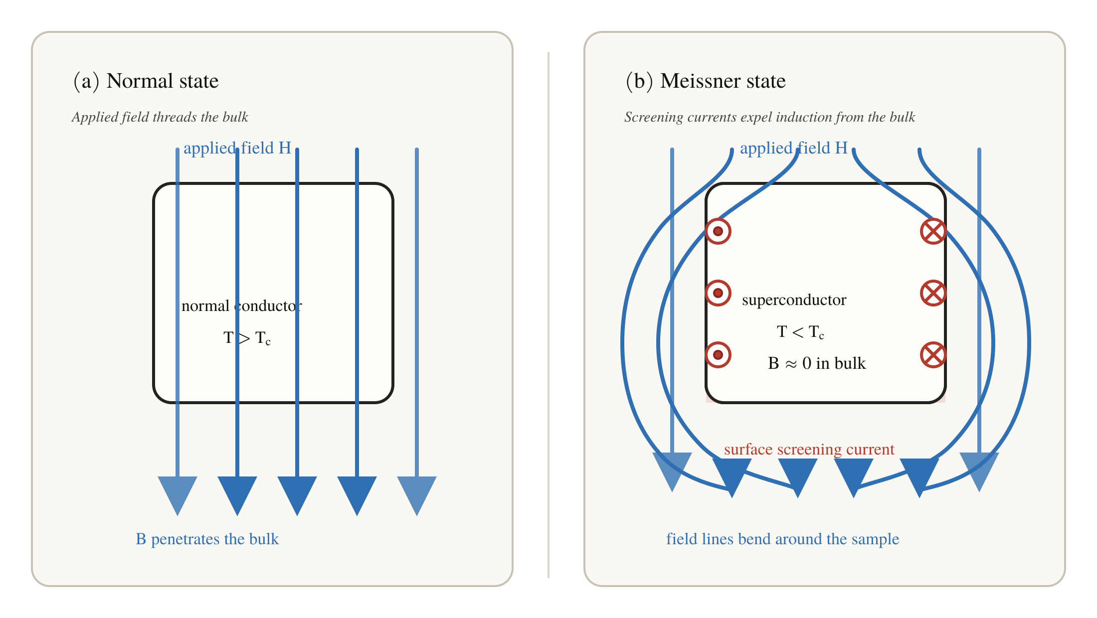
Figure 8.43: Ideal Meissner expulsion in a simply connected sample, for a Type-I superconductor with or a Type-II superconductor with . Above the applied field threads the normal conductor. Below , equilibrium surface currents confined to a London penetration layer of thickness expel the magnetic induction from the bulk, leaving away from the surface.
The London equations provide the first successful phenomenology of superconducting electrodynamics. [67] Their importance is clearest when a superconductor is compared with a perfect conductor.
In the collisionless Drude limit ,
Taking the curl and using Faraday’s law,
gives
This permits frozen-in magnetic flux. It does not force flux expulsion, because the integration constant is set by the magnetic history of the sample.
The London generalisation is to replace this history-dependent perfect-conductor behaviour by an equilibrium constitutive relation for the superconducting state:
Equivalently, the superconducting current is tied directly to the gauge field in a phase-rigid condensate, so that the equilibrium state screens the magnetic induction rather than merely preserving its initial value. Combining this with Ampère’s law,
and taking another curl gives
Magnetic field therefore decays exponentially into the sample over the penetration depth . London theory captures the Meissner effect and introduces the first intrinsic superconducting length scale. [70, 71]
Ginzburg and Landau introduced a phenomenological theory of superconductivity in terms of a complex order parameter
[68] Above the transition , while below it . The symbol is a coarse-grained condensate field, not a single-particle wavefunction; is proportional to the superfluid density in the simplest normalisation, and is the macroscopic superconducting phase.
A minimal GL free-energy functional is
where is the normal-state reference free energy, changes sign at the transition, stabilises the ordered state, and are the effective mass and charge of the condensate degree of freedom, is the electromagnetic vector potential, and is the magnetic induction. The quadratic and quartic terms set the local condensation energy, the covariant-gradient term penalises spatial phase or amplitude variations and couples the condensate to electromagnetism, and is the magnetic-field energy. The amplitude encodes condensate strength, while the phase controls currents and gauge coupling.
Varying with respect to and gives
and
GL theory introduces two characteristic lengths:
The first controls magnetic screening; the second controls how rapidly the order parameter heals after a perturbation. Later chapters reuse exactly this phase-amplitude language, but for multicomponent condensates rather than a single complex scalar.
Gor’kov later derived GL theory from BCS theory near , placing the phenomenology on a microscopic footing. [19]
The ratio
determines the magnetic character of the superconductor.
For the material is Type I: It remains in the Meissner state up to a critical field. For the material is Type II: Magnetic flux penetrates above a lower critical field in the form of vortices while superconductivity survives up to an upper critical field.
Around a vortex the condensate phase winds by , the order parameter is suppressed in the core, and the defect carries quantised magnetic flux. Abrikosov showed that these vortices form regular lattices. [72, 61]
The Type I/Type II distinction is the first place where the phase stiffness, magnetic screening, and topological defects of the condensate appear together in a single framework.
Single-valuedness of the complex order parameter produces a global quantisation condition. Around a closed loop ,
In equilibrium away from singularities,
Using Stokes’ theorem,
Experiments by Doll–Näbauer and Deaver–Fairbank found , giving direct evidence that the superconducting carriers have charge . [73, 74] The theoretical interpretation is not limited to those early low-temperature samples. Byers and Yang showed that the flux response of a superconducting cylinder is fixed by gauge invariance and the global phase of the many-body state, while later measurements in high- materials found the same flux quantum . [75, 76] This universality is why flux quantisation is treated as evidence for a coherent charge- condensate rather than as a material-specific detail.
Flux quantisation is not an incidental effect. It is the global expression of condensate phase coherence and will later reappear when relative phases and loop variables are introduced inside a unit cell.
The microscopic theory of conventional superconductivity was established in three steps:
The detailed algebra is deferred to the appendices. Only the structural results are needed here.
Electrons repel through the Coulomb interaction, but in a metal that interaction is screened. In addition, lattice vibrations can mediate an effective attraction in a narrow shell near the Fermi surface, typically set by a phonon scale such as . Pairing is therefore a low-energy effective interaction rather than a bare microscopic attraction.
Consider two electrons above a filled Fermi sea with opposite momenta and energies
Suppose the interaction is attractive only in a thin shell near the Fermi surface,
for
and vanishes outside that shell. Solving the two-body problem in the presence of the Fermi sea gives a bound state with binding energy
in the weak-coupling limit.
The qualitative conclusion is the important one: any arbitrarily weak attraction in the Cooper channel destabilises the Fermi sea. Superconductivity is therefore a Fermi-surface instability. [61]
BCS theory describes the superconducting state as a coherent many-body state of paired electrons. [18] The standard variational ground state is
with
The theory yields a gapped quasiparticle spectrum and a collective condensate phase. Superconductivity is therefore not a gas of independent bound pairs, but a coherent many-body state with long-range phase order.
At the mean-field level, the same four-fermion interaction can be reorganised into distinct contraction channels. For the present chapter the important contrast is between direct density renormalisation (Hartree), exchange renormalisation (Fock), ordinary Cooper pairing in the BCS channel, and the anomalous Gor’kov structure that appears once particle number is not fixed term-by-term in the paired description.

BCS theory is supported by several standard observations. The excitation gap appears in tunnelling spectroscopy and in activated low-temperature thermodynamics. [77] Coherence effects appear in phenomena such as the proximity effect and the Hebel–Slichter peak. [78, 79, 80] The isotope effect shows that lattice dynamics enter the pairing interaction in conventional superconductors. [81, 82]
These results matter here only as the minimal microscopic theory needed for what follows. Later chapters will keep the condensate language but generalise the internal structure of the order parameter.
The supercurrent is controlled by the gauge-invariant phase gradient,
A stationary supercurrent therefore does not require an electric field in the same way as normal-state transport. This is the low-energy expression of phase rigidity.
The same structure explains magnetic screening. The GL kinetic term
implies that once the condensate amplitude is nonzero, the electromagnetic field becomes massive within the medium and magnetic field decays over the scale . In condensed-matter language this is the Anderson mechanism. [23, 83, 84]
Writing
identifies as the phase fluctuation and as the amplitude fluctuation. For a global broken symmetry the phase mode would be gapless. With dynamical electromagnetism included, that mode is absorbed into the gauge sector, while the amplitude mode remains gapped. [85, 86, 83, 84]
Josephson relations and internal relative-phase dynamics are deferred to Chapter 4, where they are needed in the multicomponent setting relevant to the thesis mechanism.
This chapter has set the conventional baseline for the thesis. The central lesson is that superconductivity is not just a metal with infinite conductivity: it is an equilibrium condensate with phase rigidity, gauge coupling, magnetic screening, and quantised circulation. The Meissner effect, London penetration depth, GL order parameter, vortices, and flux quantum are different expressions of this same charged coherent state.
The microscopic BCS picture supplies the complementary low-energy view. Pairing is organised by the Fermi surface, and the superconducting order parameter is a collective field built from electronic pair correlations. In the simplest single-component case, the phase mostly controls electromagnetic response and supercurrent. In the multicomponent systems studied later, however, relative phases, orbital structure, spin structure, and internal winding can become independent variables in the free energy. That is the point of carrying the conventional framework forward: it provides the reference language against which time-reversal-symmetry breaking, loop-supercurrent order, and internally structured pairing can be identified.
Supporting derivations of the Cooper instability, the BCS variational state, Anderson pseudospins, and the geometric form of GL theory are collected in the appendix chapter on conventional superconductivity derivations.
This chapter provides the BdG symmetry and topological language used later to analyse microscopic representatives of internally winding TRSB states, including SSH-type lattice models. The aim is not a general survey of topological condensed matter. Only the structures used later are retained: intrinsic BdG constraints, physical time-reversal and chiral symmetries, the relevant Altland–Zirnbauer (AZ) classes, the corresponding invariants in , and the boundary-state logic needed for later microscopic modelling.
The methodological order is symmetry first. One fixes the BdG symmetry algebra, identifies the corresponding AZ class, computes only the invariants available in that symmetry class and dimension, and then interprets edges, domain walls, vortices, or impurity-induced boundaries. The 2D SSH-type model enters precisely for this reason. It provides a controlled lattice representative in which chiral symmetry, winding structure, and boundary localisation are transparent before superconducting pairing is added.
The workflow used later is to fix the physical symmetry content, especially whether TRS is preserved or broken, then write the corresponding BdG Hamiltonian with its intrinsic particle-hole constraint, identify the AZ class from the BdG symmetry algebra, compute only the invariant appropriate to that class and dimension, and interpret boundary or defect states from the invariant rather than from model-specific intuition alone.
This matters directly for internally winding TRSB states. A state that preserves physical TRS belongs to a different BdG class from one of its TRSB partners. Once the loop-current chirality is selected, the symmetry class changes, and so does the available topological diagnostic.
Crystal symmetry enters effective Hamiltonians at several levels. A point group records the rotations, mirrors, and inversions that leave a chosen point fixed. It controls the transformation of local objects such as orbitals, spin components, angular momentum, and onsite order parameters. A space group adds translations to these point-group operations. If an operation combines a point-group action with a fractional translation, the space group is nonsymmorphic. Such operations can enforce band sticking and degeneracies at high-symmetry momenta or along high-symmetry lines, so they cannot always be replaced by ordinary point-group reasoning.
At a particular momentum , the relevant symmetry is the little group of : the subset of crystal operations that maps back to itself up to a reciprocal lattice vector. The little group constrains band degeneracies and the allowed form of the low-energy Hamiltonian near that momentum. Thus a material-specific tight-binding or Wannier Hamiltonian is not just a fit to band energies; it must preserve the symmetry representation content of the low-energy states.
The local states, momentum polynomials, spin components, and order-parameter components can be classified by irreducible representations of the relevant point group or little group. A term is symmetry-allowed if the full product of all its factors transforms as the totally symmetric representation. Equivalently, the term must be a scalar under all operations in the symmetry group.
For a normal-state Bloch Hamiltonian, covariance under a crystal operation means
where acts on the internal orbital, sublattice, and spin degrees of freedom. If a term is written as
then it is allowed only when
for every symmetry operation . In representation language, this is precisely the statement that the combined object transforms as the identity representation.
The same symmetry-first logic also controls which microscopic or effective Hamiltonian terms may be written before any topological invariant is computed. The standard invariant method is to assign each factor in a proposed term to a representation of the crystal point group and then keep only products that contain the totally symmetric representation [87, 88]. For a term written schematically as
where is a momentum form factor, acts in an orbital or sublattice subspace, and acts on spin, the term is allowed only if
in the appropriate point-group notation. The same construction underlies Landau free-energy invariants, except that the matrices are replaced by order-parameter components [89].
The distinction between polar and axial vectors is essential in spin-orbit-coupled models. Position, momentum, electric field, and crystal gradients are polar vectors. They change sign under inversion. Spin and orbital angular momentum are axial vectors. They are even under inversion because they are generated by cross products of two polar vectors, such as .
In a centrosymmetric point group this means that a momentum form factor and a spin matrix generally carry different inversion parity. A spin-dependent Hamiltonian term must therefore combine spin, orbital, and momentum factors so that the total product has even parity and transforms as the identity representation. This is why a spin-orbit term may be onsite in one orbital subspace but must be momentum-dependent in another.
This is particularly important for spin-orbit coupling. Spin transforms as an axial vector, like angular momentum, not as a polar vector. Therefore a spin-dependent hopping, hybridisation, or pairing term must carry whatever orbital and momentum transformation character is needed to make the full product a scalar. In multiorbital models, an apparently artificial Pauli-matrix structure such as an imaginary interorbital spin-flip term can be the low-energy remnant of an atomic spin-orbit matrix element or of downfolding from a larger orbital manifold [90]. Later, this invariant-method logic is used to distinguish a symmetry-allowed diagnostic texture from a material-specific claim about a particular Wannier Hamiltonian.
For example, in an orthorhombic setting the spin matrix transforms as the axial-vector component . With the conventional assignment
an onsite interorbital spin-orbit term is allowed only if
Equivalently, the orbital matrix itself must transform as . If the corresponding term is momentum dependent,
the invariant condition becomes
BdG Hamiltonians possess an intrinsic particle–hole constraint because the Nambu basis is redundant. Let be a BdG Hamiltonian in Nambu space. There exists an antiunitary operator
such that
This implies a spectrum symmetric about zero energy and eigenstates in pairs.
The important conceptual point is that this particle–hole relation is intrinsic to the BdG description. It is not an optional microscopic symmetry in the same sense as physical TRS.
Time-reversal symmetry is an optional physical symmetry. When present, it imposes
For spin- electrons, one typically has .
This distinction is used repeatedly later. Preserving TRS keeps the system in a time-reversal-invariant BdG class. Selecting one of two internally winding TRSB partners removes that symmetry and shifts the topological classification accordingly.
When both TRS and the AZ particle–hole symmetry are present, their product defines a unitary chiral symmetry operator obeying
Chiral symmetry is often the cleanest route to winding-number invariants because it allows an off-diagonal form
A standard classification step is spectral flattening:
performed without closing the bulk gap or breaking the symmetry algebra. Topology is then the homotopy class of the flattened Hamiltonian subject to the same symmetry constraints. [8, 9, 91]
The periodic table of free-fermion phases is a stable classification. The word stable means that adding trivial, decoupled bands does not change the topological phase. This is why the classification is naturally stated in K-theoretic language: it organises gapped Hamiltonians modulo the physically harmless operation of adjoining inert degrees of freedom. [8, 91]
Only a small subset of the periodic table is used later. The recurring BdG classes are BDI, D, and DIII. Other classes can appear when additional spin-rotation constraints are imposed, but they are not the main diagnostic cases for the thesis.
| BdG AZ class | TRS | PHS | CS | Main later use | |||
|---|---|---|---|---|---|---|---|
| BDI | yes | chiral winding in 1D and in momentum-resolved 1D cuts of SSH-type models | |||||
| D | no | TRSB BdG Hamiltonians, Chern phases, and chiral boundary structure | |||||
| DIII | yes | time-reversal-invariant reference class before TRS is broken |
Here TRS means , TRS means , and PHS refers to in the AZ sense. The periodicity of the full table is the familiar Bott periodicity of the stable classification, but the later chapters only need the subset displayed above. [92, 8, 9, 91]
If chiral symmetry allows an off-diagonal block form
then the winding number is
This integer invariant controls the number of protected zero modes at a boundary as long as the chiral symmetry is maintained. It is the basic topological diagnostic for SSH-type representatives and for fixed-momentum cuts of the 2D model discussed below. [9, 91]
For a fully gapped 2D BdG system without TRS, the relevant invariant is the Chern number of the occupied BdG bands:
with the Berry curvature of the negative-energy eigenspace. Nonzero implies chiral boundary structure. In superconducting language this means chiral Majorana edge modes counted by the net chirality. [92, 8]
In class D, the 1D invariant is . In class DIII, one obtains indices in and an integer winding invariant in . The detailed formulas are not needed repeatedly in the later chapters, but the interpretive rule is: preserving TRS keeps one in a DIII-type setting, while selecting a TRSB partner generally moves the system into class D and replaces helical boundary logic with chiral boundary logic.
A bulk invariant constrains boundaries and defects. In BdG systems the physically important boundaries are often not sample edges but vortices, domain walls, Josephson interfaces, and impurity-generated internal boundaries. The same symmetry-first logic applies to all of them: if the invariant changes across an interface, low-energy boundary states are expected. [93, 91]
This point is especially relevant to internally winding TRSB states, because the natural defects are domain walls between opposite loop chiralities and interfaces where the internal phase structure changes.
The periodic table classifies fully gapped phases. Nodal BdG Hamiltonians can still be topological when nodes carry their own topological charge. In three dimensions, isolated point nodes act as Weyl nodes and enforce surface arcs connecting their surface projections. This distinction between gapped and nodal topology is kept here only because later boundary-state reasoning requires it; the present chapter does not attempt a general review of nodal superconductors. [94, 95, 96]
The SSH material is included because it is part of the later modelling logic, not as a generic pedagogical detour. SSH-type lattices provide controlled representatives for chiral symmetry, winding numbers, and boundary localisation. Once embedded into BdG form, the same lattices become useful representatives for superconducting boundary states and for internally structured TRSB constructions.
The SSH chain is the canonical 1D chiral lattice model. In momentum space it may be written as
with sublattice operator
The winding number distinguishes the two dimerisation patterns, and a domain wall between them binds a midgap boundary state. This is the simplest example of symmetry-protected boundary localisation.
For later use it is convenient to keep a concrete 2D representative. A standard four-orbital square-lattice model has Bloch Hamiltonian
with
Chiral symmetry is explicit in this block-off-diagonal form. [97, 11]
The useful viewpoint is dimensional reduction. For fixed , the 2D model becomes a family of 1D chiral Hamiltonians indexed by transverse momentum. Edge states on an -normal boundary are then controlled by the momentum-resolved winding number
Boundary bands appear precisely over those values of for which the reduced 1D problem is topological.
This is why the 2D SSH-type model is useful later. It gives a controlled lattice representative for chiral symmetry, winding structure, and boundary-state analysis, and it does so in a form that can be upgraded systematically to BdG Hamiltonians.
To connect SSH edge logic to superconducting boundary physics, embed the model into BdG form by introducing a chemical potential and pairing:
This automatically satisfies the intrinsic BdG particle–hole constraint. Depending on the pairing structure and on whether physical TRS is preserved, the resulting Hamiltonian may fall into class BDI, D, or DIII.
The dimensional-reduction logic survives the BdG embedding. Fixing again produces a family of 1D BdG Hamiltonians. Over ranges of these reduced Hamiltonians can be topological, implying boundary-localised Majorana bands, flat bands, or arc-like structures depending on which symmetries remain and whether the bulk is gapped or nodal.
This makes the SSH-type model a useful controlled representative for later microscopic analysis. It is a lattice setting in which symmetry classification, winding structure, and boundary consequences can be followed explicitly before additional ingredients such as internally winding TRSB order are introduced.
The role of topology in the thesis is now fixed. BdG Hamiltonians carry an intrinsic particle–hole constraint, while physical TRS and chiral symmetry determine the AZ class and hence the relevant invariant. The later chapters primarily use the BDI, D, and DIII sectors of the periodic table, together with winding and Chern diagnostics and the associated bulk–boundary logic.
The SSH material is included because it supplies a controlled lattice representative for this programme. In particular, the 2D SSH-type model is used later as a symmetry-clean representative for winding structure, boundary-state analysis, and superconducting BdG extensions relevant to internally winding TRSB states.
The detailed representation bookkeeping used for later orthorhombic multiorbital Hamiltonians is collected in the appendix chapter on representation bookkeeping.
Mean-field theory replaces an interacting fermion Hamiltonian by a quadratic (Gaussian) variational Hamiltonian whose parameters are fixed by self-consistency:
The quadratic problem can be solved exactly (diagonalised), and all required expectation values are computed within that Gaussian reference state.
For superconducting order this is the standard route from BCS and Gor’kov mean-field theory to the BdG equations and their de Gennes real-space formulation, while in lattice-model language the same closure yields Hartree, Fock, and pairing channels for Hubbard-type and multiorbital interactions. [18, 19, 78, 14, 15, 16]
Throughout we keep the fixed tensor-product bookkeeping
where (\mathcal H_{\mathrm{int}}=\mathrm{span}{|m\rangle : m\in\mathscr M}) denotes the internal or orbital one-body space.
We therefore present each object first in compact tensor notation and then in explicit indices, consistent with the symmetry/tensor construction of the preceding chapters.
This section fixes once-and-for-all the translation between explicit indices and operator/tensor (Kronecker) notation.
Let the physical (non-Nambu) one-body space be
and introduce a composite index
Collect annihilation operators into a column vector (\hat c) over (\mathcal H_1),
The equal-time correlators needed for self-consistency are then
In operator language, (ρ) and (χ) are matrices on (\mathcal H_1), i.e. (ρ,χ\in \mathrm{End}(\mathcal H_1)).
If (A) acts on (\mathcal H_{\mathrm{lat}}) and (B) on (\mathcal H_{\mathrm{spin}}), then
acts on (\mathcal H_{\mathrm{lat}}\otimes\mathcal H_{\mathrm{spin}}), with the remaining factors understood to carry identities.
We will write identity operators as (𝟙_{\mathrm{lat}}), (𝟙_{\mathrm{Nambu}}), etc., and use a Pauli basis ({τ_\ell}) on Nambu space and ({σ_j}) on spin space:
It is also convenient to define raising/lowering combinations
so that Nambu block matrices can be written compactly as sums of Kronecker products.
In real-space/orbital/spin indices, the transpose (T) means swapping the composite indices:
Equivalently, introduce the swap operator (𝒫) on (\mathcal H_1\otimes\mathcal H_1) defined by
Then “antisymmetry under exchange” is expressed by the antisymmetriser (𝒜=(𝟙-𝒫)/2). In particular, fermionic antisymmetry of the pairing channel will be written as
i.e. (𝒫) projects out symmetric components in the combined indices.
Introduce the Nambu spinor on the doubled one-body space (\mathcal H_{\mathrm{Nambu}}\otimes\mathcal H_1),
Then any quadratic BdG mean-field Hamiltonian can be written as
where (\boldsymbol{\mathcal H}^{\mathrm{MF}}) is a Hermitian matrix acting on (\mathcal H_{\mathrm{lat}}\otimes\mathcal H_{\mathrm{Nambu}}\otimes\mathcal H_{\mathrm{int}}\otimes\mathcal H_{\mathrm{spin}}), and (\mathcal E_{\mathrm{gs}}) is the mean-field ground-state (double-counting) constant.
In Nambu block form,
where (\boldsymbolΣ) collects all normal self-energies (Hartree/Fock-like) and (\boldsymbolΔ) is the anomalous (pairing) mean field. This is the standard Gor’kov/de Gennes BdG structure written in the tensor conventions used throughout the thesis. [19, 78]
A compact Kronecker representation of this BdG structure is
where (\boldsymbol h^{\mathrm{MF}}) and (\boldsymbolΔ) act on (\mathcal H_1) and the (τ)-matrices act on (\mathcal H_{\mathrm{Nambu}}).
To maintain continuity with the shift/tensor template, expand (\boldsymbol{\mathcal H}^{\mathrm{MF}}) in a basis on the internal/Nambu/spin factors, with lattice operators as coefficients:
where ({τ_\ell}) is a Pauli basis on (\mathcal H_{\mathrm{Nambu}}), ({λ_i}) is a Hermitian operator basis on (\mathcal H_{\mathrm{int}}), ({σ_j}) is a Pauli basis on (\mathcal H_{\mathrm{spin}}), and (\mathbb X_{\ell i j}) are operators on (\mathcal H_{\mathrm{lat}}) (typically built from masked shifts, projectors, or inhomogeneous geometry operators).
This viewpoint emphasises that the mean-field problem remains “quadratic plus symmetry constraints”: once a symmetry generator set is chosen, the allowed channels (τ_\ell\otimesλ_i\otimesσ_j) are constrained exactly as in the free-fermion construction, while the lattice coefficients (\mathbb X_{\ell i j}) are determined self-consistently.
In explicit indices, the most general quadratic mean-field interaction on an arbitrary lattice (Ω) can be written as
Here (\symbf ρ) is Hartree-like (density) renormalisation, (\symbf Φ) is Fock-like (exchange/hopping renormalisation), and (\symbf Δ) is Gor’kov-like pairing. These channels exhaust the Wick contractions of a two-body interaction into quadratic (Gaussian) fields.[^1] In model Hamiltonians this is precisely the decomposition used for on-site and extended Hubbard interactions, as well as for multiorbital Kanamori-type local interactions. [14, 15, 16]
It is sometimes useful to recognise these as kernels on (\mathcal H_1):
with the precise identification fixed by the chosen microscopic interaction tensor (\symbf U) and by the “diagonal vs off-diagonal” decomposition in the chosen basis.
For the full interacting Hamiltonian (\hat{\mathcal H}=\hat{\mathcal H}_0+\hat{\mathcal H}I), the exact free energy is Mean-field theory approximates this by evaluating the expectation values in the Gaussian (quadratic) reference ensemble generated by (\hat{\mathcal H}^{\mathrm{MF}}{\mathrm{BdG}}):
Writing
one obtains the standard decomposition
Stationarity (saddle-point) of (F) with respect to the variational fields yields the self-consistency equations.[^2]
Conceptually, mean-field theory minimises the exact free-energy functional over the restricted family of Gaussian density matrices:
This restriction is precisely what makes Wick factorisation exact inside the trial ensemble, and what turns the interacting problem into a closed fixed-point problem for the quadratic kernels (Σ) and (Δ). In the superconducting context this restricted variational logic is the standard mean-field closure behind BdG theory. [18, 78]
For a density–density interaction (schematically (\hat{\mathcal H}_I=\sum U,\hat n\hat n)), Wick’s theorem gives, in explicit indices,
The exchange minus sign is enforced by fermionic anticommutation.
In composite-index language, a typical (model-dependent) rewriting is
where (U_{\alpha\beta}) is the interaction kernel in the (|\alpha\rangle) basis (site/orbital/spin).
To evaluate these expectation values systematically we introduce Matsubara kernels (imaginary-frequency resolvent kernels), rather than real-frequency Green’s functions.
Define the imaginary-time Nambu kernel
where (\hatΦ(τ)=e^{τ \hat{\mathcal H}^{\mathrm{MF}}{\mathrm{BdG}}}\hatΦ e^{-τ \hat{\mathcal H}^{\mathrm{MF}}{\mathrm{BdG}}}) and (\mathsf T_τ) is imaginary-time ordering.
The fermionic Matsubara components are
For a quadratic mean-field Hamiltonian, the kernel is the matrix inverse (imaginary-frequency resolvent)
This is the Matsubara analogue of the resolvent: it is the unique object from which all bilinear correlators follow by frequency summation (or integration at (T=0)). This is just the imaginary-frequency Green-function formulation of the same BdG mean-field problem. [19, 78]
Let (\boldsymbol{\mathcal H}^{\mathrm{MF}}Ψ_r=\mathcal E_rΨ_r). The intrinsic BdG particle–hole symmetry implies a paired spectrum (\pm \mathcal E_r). The resolvent kernel has the spectral representation
where (\barΨ_r) is the particle–hole conjugate of (Ψ_r) (defined precisely below).
Write the Nambu kernel in block form
where (\mathcal K) is the normal (particle–particle) kernel and (\mathcal L) is the anomalous (pairing) kernel. In Kronecker language, this block structure corresponds to the decomposition in (τ)-space.
In explicit indices (site (\mathbf i,\mathbf i’), spin (σ,σ’), orbitals (m,m’)), write (Ψ_r=((u_{\mathbf iσ m})r,(v{\mathbf iσ m})_r)). Then
and
Define the transpose in the combined non-Nambu indices by
Intrinsic BdG particle–hole symmetry implies the block relations
so that
For self-consistency we require normal and anomalous equal-time correlators:
These follow from the Matsubara kernels by
and in explicit indices,
Carrying out the Matsubara sums using the spectral representation yields the familiar BdG-eigenvector formulas at finite temperature:
At finite temperature the Matsubara frequencies are discrete,
In the zero-temperature limit (β\to\infty), Matsubara sums become imaginary-frequency integrals:
so one may compute observables directly from (\boldsymbol{\mathcal K}(iω)) without analytic continuation to real frequency.
Equivalently (and most usefully in BdG numerics), equal-time correlators become projectors onto the occupied (negative-energy) BdG subspace. Define the occupied projector
In Nambu block form this projector has the universal structure
where the transpose is taken in the combined non-Nambu indices. Thus (ρ) and (χ) may be obtained either from the imaginary-frequency integral formula above or directly from (𝒫_-). In explicit indices (including negative-energy eigenvectors),
which is precisely the (T\to0) limit of the finite-(T) Fermi-factor formulas, (f(\mathcal E)\to Θ(-\mathcal E)).
The variational stationarity condition (\delta F=0) yields
The resulting saddle-point equations can be expressed compactly as “interaction tensor (\times) densities”.
Write the microscopic interaction kernel as a tensor (U) in the composite basis,
Introduce the diagonal-extraction superoperator (𝒟) (in the chosen local basis) defined by
and recall that matrix transpose is ((A^T){\alpha\beta}=A{\beta\alpha}).
Then the three mean-field channels may be represented schematically as
with the understanding that “(U)” here denotes the appropriate contraction of interaction indices with the density matrices in the same basis used to define (U_{\alpha\beta}). This tensor form makes the physics transparent: Hartree couples to the diagonal density, Fock to exchange (transpose), and pairing to the anomalous correlator.
The intrinsic fermionic antisymmetry constraint (independent of TRS) is
i.e. only antisymmetric components in combined indices contribute to pairing.
In explicit-index form (as used throughout your construction),
The symmetry (\symbf{U}{\mathbf{i},\mathbf{j},σ,τ,m,n}= \symbf{U}{\mathbf{j},\mathbf{i},τ,σ,n,m}), together with fermionic algebra, implies in common gauges
The resulting mean-field Hamiltonian is therefore
Before turning to spatially inhomogeneous textures, it is useful to examine the same self-consistency equations in uniform bulk settings. Even in this simplest limit, the fixed-point problem already shows the characteristic separation between weak, intermediate, and strong coupling, together with a strong dependence on the underlying normal-state density of states. This is the usual BCS-to-strong-coupling mean-field phenomenology for attractive lattice models. [18, 15]
Illustrative two-dimensional bulk BCS benchmark showing the self-consistent zero-temperature gap as a function of interaction strength for chemical potential . The weak-coupling regime is exponentially suppressed, the intermediate regime marks the rapid onset of pairing, and the strong-coupling regime crosses over toward large local pair formation.
Bulk BCS temperature and density-of-states comparison for simple one-, two-, and three-dimensional model dispersions. The left panel shows the self-consistent gap decreasing toward the critical temperature in each dimension, while the right panel shows how differences in the normal-state density of states help set the pairing scale and the most favorable chemical-potential window.
Mean-field theory corresponds to a saddle point of the variational free-energy functional restricted to Gaussian density matrices. To go beyond static mean-field theory, we expand the free energy to quadratic order in fluctuations of the mean fields. This yields a controlled description of collective modes (RPA, Anderson–Bogoliubov, amplitude modes, etc.) and provides the starting point for diagrammatic and numerical extensions. In superconductors this is the standard route from static BdG mean field to RPA/Gaussian collective-mode theory. [23, 83, 78]
Throughout this section, all indices and tensor placements follow the conventions fixed above.
Write the BdG kernel as a saddle-point value plus fluctuations:
In Nambu block form,
where
represent fluctuations in the normal and anomalous channels.
In composite-index notation,
We group all fluctuating fields into a single vector:
with the understanding that symmetry constraints (Hermiticity, antisymmetry) are enforced either explicitly or by restricting the independent components.
The mean-field free energy may be written as
where the trace includes Matsubara frequency, Nambu space, and (\mathcal H_1).
Expanding to second order about the saddle point,
The linear term is
where
Using the saddle-point equations derived above, one has
which is simply the statement that mean-field theory is stationary.
The quadratic fluctuation action is
This has a universal structure:
where (\mathcal M) is the Gaussian fluctuation kernel (inverse propagator of collective modes).
Write the trace explicitly:
Separating normal and anomalous parts gives three types of contributions:
These expressions are exact for Gaussian fluctuations.
The interaction part contributes a local quadratic form:
with
Combining fermionic loops and interaction terms yields the standard RPA / Gaussian-fluctuation kernel
where (\Pi) is the generalized susceptibility matrix constructed from two BdG propagators. This is the superconducting analogue of the usual RPA inverse propagator, now written in Nambu-channel form. [23]
Define a collective-channel index (A=(\alpha\beta,\mu)) with
Then
where the vertex matrices are
At zero external frequency ((Ω_m=0)), this kernel controls static stability; its zeros correspond to Goldstone modes and instabilities.
In the superconducting case this reproduces the familiar Anderson-Bogoliubov phase mode and its gauge-coupled descendants. [23, 83]
This formulation is directly compatible with sparse real-space BdG codes and symmetry-restricted tensor constructions.
Solve the BdG eigenproblem
with components (u_r={(u_{\mathbf iσ m})r}) and (v_r={(v{\mathbf iσ m})_r}). The corresponding Bogoliubov quasiparticles (\hatγ_r) diagonalise the quadratic Hamiltonian:
with the (\pm\mathcal E_r) pairing enforced by intrinsic BdG particle–hole symmetry. This is the standard Bogoliubov quasiparticle construction in the de Gennes formulation. [78]
This section treats time-reversal symmetry (TRS) as an optional physical symmetry constraint on (\boldsymbol{\mathcal H}^{\mathrm{MF}}), and particle–hole symmetry (PHS) as an intrinsic constraint of the BdG/Nambu representation.
Let (\hat{\mathcal C}) denote complex conjugation in the chosen basis. For spin-(\tfrac12) electrons define the antiunitary time-reversal operator on (\mathcal H_1),
In real space,
and in translation-invariant systems TRS flips momentum (\mathbf k\mapsto -\mathbf k).
On BdG/Nambu space, take the induced unitary part acting diagonally in particle/hole components:
TRS of the BdG mean-field Hamiltonian is then the conjugation constraint
In Nambu blocks this implies
where (U_{\mathsf T}=𝟙_{\mathrm{lat}}\otimes 𝟙_{\mathrm{int}}\otimes(-iσ_y)) acts on the non-Nambu factors.
Using the expansion
TRS becomes a selection rule on allowed channels:
and the lattice operators (\mathbb X_{\ell i j}) must satisfy the corresponding relations (including (\mathbf k\mapsto -\mathbf k) if applicable). In practice this is the cleanest way to enforce TRS while building a symmetry-adapted mean-field ansatz. This is also the natural language used in symmetry classifications of unconventional superconducting order parameters. [25]
BdG Hamiltonians possess an intrinsic antiunitary particle–hole symmetry because the Nambu basis is redundant. Define
with unitary part (U_{\mathsf C}=𝟙_{\mathrm{lat}}\otimes τ_x\otimes 𝟙_{\mathrm{int}}\otimes 𝟙_{\mathrm{spin}}). The intrinsic BdG constraint is
Consequently, if (\boldsymbol{\mathcal H}^{\mathrm{MF}}Ψ=EΨ), then (\barΨ:=U_{\mathsf C}Ψ^) satisfies (\boldsymbol{\mathcal H}^{\mathrm{MF}}\barΨ=-E\barΨ), explaining the (\pm E) pairing of the BdG spectrum. In components, this corresponds to the familiar mapping ((u,v)\mapsto(-v^,u^*)) (up to Nambu convention).
Independently of TRS, fermionic antisymmetry imposes antisymmetry of the pairing kernel under exchange of combined indices:
In swap-operator language this is (𝒫,Δ,𝒫=-Δ), i.e. (Δ) lives in the antisymmetric sector selected by (𝒜).
Recall
From TRS one obtains
and from intrinsic BdG PHS,
These kernel constraints are the Matsubara-resolvent versions of the usual BdG symmetry relations and imply the block identities used above, such as (\bar{\mathcal K}(iω_n)=-\mathcal K(-iω_n)^{\mathrm T}) and (\bar{\mathcal L}(iω_n)=\mathcal L(iω_n)^\dagger).
Mean-field BdG theory and Kohn–Sham (KS) density-functional theory share a common structural theme—both solve a self-consistent quadratic problem—but differ in what is taken as fundamental and what is approximate.
Mean-field theory may be viewed as a restricted variational problem: one minimises the exact free-energy functional over the subset of density matrices generated by quadratic trial Hamiltonians,
leading to saddle-point (self-consistency) equations for (Σ) and (Δ). The microscopic interaction tensor (\symbf U) explicitly determines which channels appear and how they couple.
Ground-state DFT asserts that the ground-state density determines the external potential (up to a constant), and that the ground-state energy may be written as a universal functional of the density [98]. The KS construction introduces a non-interacting auxiliary system that reproduces the interacting density [99]. In lattice language one may write schematically
with (v_{xc,\mathbf i}[n]=\delta \mathcal F_{xc}/\delta n_{\mathbf i}). Thus the form of the quadratic problem resembles Hartree-like self-consistency, but the interpretation is different: interactions are encoded in universal functionals rather than via decoupling a chosen microscopic (\symbf U).
Because the present derivation is explicitly at finite temperature, the closest DFT analogue is Mermin’s extension of DFT to thermal ensembles, formulated as a variational principle for the free energy [100]. This is the clean point of contact: both approaches are naturally expressed at the level of a thermodynamic potential and solved by self-consistent Euler–Lagrange equations, though the underlying functionals and approximations differ.
Superconducting DFT extends DFT by enlarging the basic variables to include an anomalous (pair) density (χ(\mathbf r,\mathbf r’)=\langle \hatψ_\downarrow(\mathbf r)\hatψ_\uparrow(\mathbf r’)\rangle), leading to KS-like equations with a BdG structure [101]. This gives a clean mathematical mapping to self-consistent BdG, but only at the level of the fixed-point equations. The two theories are not equivalent: their Nambu matrices can be written in the same form, but the entries are generated by different closures.
On the SCDFT side one solves a superconducting Kohn–Sham problem of the form
Here both the normal KS operator and the pairing field are functionals of the normal and anomalous densities. In continuum language one may write schematically
and the densities are reconstructed self-consistently from the quasiparticle amplitudes. This is the superconducting analogue of the KS construction: the quadratic auxiliary problem is chosen so as to reproduce the interacting densities, not because the electrons are assumed to interact only through a particular microscopic model tensor.
By contrast, the self-consistent BdG problem developed in this chapter starts from a chosen low-energy Hamiltonian and a chosen interaction tensor (\symbf U). After mean-field decoupling one obtains
with (ρ_{\alpha\beta}=\langle \hat c^\dagger_\beta \hat c_\alpha\rangle) and (χ_{\alpha\beta}=\langle \hat c_\beta \hat c_\alpha\rangle) exactly as in the rest of this chapter. In the simplest pairing-only closure this is just the usual gap equation (Δ\sim -U,χ), while Hartree and Fock corrections sit in (Σ_{\mathrm{MF}}[ρ]).
Once both theories are expanded in a finite localized basis, the algebraic correspondence is immediate:
Normal density maps to the Hartree/Fock density matrix, anomalous density maps to the pair amplitude, the KS pairing field maps to the BdG gap matrix, and the KS normal potential maps to the mean-field normal Hamiltonian. This is why a Wannier-basis KS-BdG calculation and a multiorbital lattice BdG calculation can look almost indistinguishable numerically even though they arise from different theories.
The decisive difference is the origin of the self-consistency closure. In SCDFT, the pairing field arises in principle from an exchange-correlation functional derivative with respect to the anomalous density,
and the normal KS potential likewise comes from functional derivatives with respect to the normal density [101]. In model BdG, by contrast, the gap and self-energy come from the explicit decoupling of a chosen microscopic interaction tensor (\symbf U). One may therefore regard self-consistent BdG as a restricted KS-BdG-shaped fixed-point problem with a model closure, but not as SCDFT itself.
That distinction matters physically. A lattice BdG solver is an effective low-energy mean-field theory: it is excellent for testing candidate order parameters, symmetry constraints, multiband structure, or TRSB mechanisms inside a chosen model space. It does not automatically supply the material-specific exchange-correlation pairing kernel, retardation effects, screened Coulomb physics, or full density feedback that belong to a bona fide superconducting density-functional treatment. The mathematically honest statement is therefore that self-consistent BdG and KS-BdG share a common Nambu structure, while SCDFT differs in how the normal and anomalous fields are generated.
The cleanest way to make the relation precise in the notation of this chapter is to write a finite-basis free-energy functional directly in terms of the normal and anomalous one-body densities,
Here (ρ) and (χ) are the density matrices already introduced above, while (\mathcal T_s) and (\mathcal S) are understood as the kinetic and entropic contributions of the quadratic auxiliary problem. Stationarity with respect to the Gaussian reference state then produces a KS-BdG-shaped Euler equation on the Nambu-doubled one-body space,
with
This is the finite-basis SCDFT statement relevant to the thesis: once the closure is supplied by a bona fide functional of (ρ) and (χ), the quadratic fixed-point problem solved by the code is already of KS-BdG type.
Model BdG is recovered as the special case in which one chooses a restricted approximate functional rather than a universal superconducting density functional. For example, if one writes
with a pairing contribution of the schematic form
then variation immediately gives a BdG-style closure
together with the corresponding normal self-energy from (\mathcal F_{\mathrm{normal}}^{\mathrm{model}}[ρ]). In that sense every self-consistent quadratic BdG theory can be embedded in an SCDFT-shaped variational structure; what changes from theory to theory is the choice of functional closure.
This is also the precise point at which the scope of the present codebase should be understood. Our generalized quadratic solver is already broad enough to host either kind of closure:
What it does not provide automatically is the microscopic construction of the superconducting exchange-correlation functional itself. That object still has to be supplied, approximated, or derived. So the code already contains the universal quadratic backend required by SCDFT, but SCDFT as a first-principles theory is only obtained once that functional layer is specified.
“Our narrative is by no means a recommendation of how research should be done, it simply reflects what we thought, how we acted and what we felt. However, it would certainly be gratifying if it encouraged a more relaxed attitude towards doing science.”
Gerd Binnig and Heinrich Rohrer, Nobel Lecture, December 8, 1986 [102]
Throughout, calligraphic symbols denote propagators, while boldface symbols denote variational mean-field tensors.
This chapter collects the Green’s functions associated with the Bogoliubov–de Gennes mean-field Hamiltonian and shows how physical observables are obtained from them. No reference to the variational derivation or self-consistency equations is required.
The terminology “Green’s function” traces back to George Green’s original 1828 essay. [103]
Let the Bogoliubov–de Gennes Hamiltonian satisfy
with particle–hole–symmetric spectrum (\pm\mathcal E_n).
The Nambu–Gor’kov Green’s function is defined as the resolvent
In the eigenbasis,
In superconductivity, the anomalous (pair) propagator was introduced by Gor’kov in his Green’s-function formulation of BCS theory. [104]
In Nambu space the Green’s function decomposes as
It is convenient to bundle spin and orbital indices into a single multi-index (\alpha\equiv(\sigma,m)). Then the normal and anomalous blocks admit the BdG spectral representations
The particle–hole–conjugate blocks (\bar{\mathcal G}) and (\bar{\mathcal F}) are fixed by the symmetry relations below, so we do not restate them as separate sums.
Hence the full Nambu–Gor’kov Green’s function may be written as
Experimentally accessible quantities fall into two broad classes. The first comprises single-particle spectra, which are obtained from the retarded Nambu–Gor’kov Green’s function
Physical spectra measured by probes such as ARPES and STM are extracted from the electron block (\mathcal G^R), traced over spin and orbital indices.
The second class comprises linear-response functions, obtained from retarded correlators of densities, currents, and spins,
where (\hat A) and (\hat B) may denote charge-density, current, or spin operators. Microscopically these quantities are built from products of one-particle Green’s functions, supplemented by vertex corrections when required by symmetry or conservation laws.
In a translationally invariant system,
and, up to matrix-element effects, ARPES measures (I(\mathbf k,\omega)\propto f(\omega),A(\mathbf k,\omega)). This is the momentum-resolved single-particle spectral function.
The real-space counterpart is the local density of states measured by STM/STS,
for a featureless tip density of states and weak energy dependence of the tunnelling matrix element.
In the presence of impurities, one considers the modulation of the local density of states,
The Fourier amplitude (g(\mathbf q,\omega)) is the basic quasiparticle-interference observable. In a (T)-matrix treatment, (\delta N) is controlled by (\mathcal{\mathbf G},\mathcal{\mathbf T},\mathcal{\mathbf G}) in Nambu space.
Let (\Pi^R_{ij}(\omega)) be the retarded current–current correlator (\Pi^R_{ij}(\omega)\equiv \chi^R_{j_i j_j}(\omega)). Then the conductivity follows from
where the subtraction enforces gauge invariance together with the diamagnetic term. This quantity governs both the optical conductivity and the microwave response.
The London kernel (K_{ij}) is the static long-wavelength current response,
where (K_T) is the transverse part. The temperature dependence of (\lambda(T)) is correspondingly a sensitive probe of nodal structure through the superfluid stiffness.
At optical frequencies Kerr rotation is controlled by the antisymmetric part of the optical response, commonly expressed through (\sigma_{xy}(\omega)) (from (\Pi_{xy})) together with the sample’s electrodynamics (dielectric function / refractive index). Microscopically, (\sigma_{xy}) is again a current–current Kubo response in the TRSB state.
For spin operators (\hat S^\alpha),
The Knight shift is proportional to the uniform static susceptibility, (K(T)\propto \chi^{\alpha\alpha}(\mathbf q{=}0,\omega{=}0)). The NMR relaxation rate probes the low-frequency spin response,
Neutron scattering, in turn, measures
From the grand potential (\Omega) (computable from BdG eigenvalues, equivalently (\ln\det \mathcal{\mathbf G}^{-1})), one obtains the specific heat and condensation energy via
Thermal conductivity (κ_{ij}) follows from heat-current correlators (Kubo), and (κ(T)) again strongly constrains nodal structure.
Experiments such as ZF-(\mu)SR, scanning SQUID, or Hall magnetometry probe internal fields (\mathbf B(\mathbf r)) produced by equilibrium supercurrents (\mathbf j(\mathbf r)) and/or magnetization (\mathbf M(\mathbf r)),
In BdG/quasiclassical formalisms, (\mathbf j(\mathbf r)) can be expressed directly in terms of Green’s functions (paramagnetic contribution plus diamagnetic term), so that (\mathcal{\mathbf G}\Rightarrow \mathbf j \Rightarrow \mathbf B\Rightarrow P(B)) (for (\mu)SR).
| Experimental method | Measured quantity | Theory object | Green’s-function content |
|---|---|---|---|
| ARPES | (I(\mathbf k,\omega)) | (A(\mathbf k,\omega)) | (-\frac{1}{\pi}\Im,\mathrm{Tr}_{\sigma,m},\mathcal G^R(\mathbf k,\omega)) |
| STM/STS | (dI/dV(\mathbf r,V)) | (N(\mathbf r,\omega)) (LDOS) | (-\frac{1}{\pi}\Im \sum_{\sigma,m}\mathcal G^{R,m,m}_{\sigma\sigma}(\omega;\mathbf r,\mathbf r)) |
| QPI / FT-STS | (\lvert g(\mathbf q,\omega)\rvert) | (\delta N(\mathbf q,\omega)) | (\mathcal{\mathbf G}\mathcal{\mathbf T}\mathcal{\mathbf G}) (impurity (T)-matrix) |
| Optical/microwave | (\sigma_{ij}(\omega)) | conductivity | current–current (\Pi_{ij}=\chi_{j_i j_j}) |
| Penetration depth | (\lambda(T)) | superfluid stiffness | static transverse current response (K_T) |
| Kerr rotation | (\theta_K(\omega)) | TRSB optical response | antisymmetric (\sigma_{xy}(\omega)) from (\Pi_{xy}) |
| Knight shift | (K(T)) | (\chi_s(0,0)) | spin–spin (\chi_{SS}) |
| NMR (1/T_1) | relaxation rate | low-(\omega) spin fluctuations | (\sum_{\mathbf q}\Im\chi^{+-}(\mathbf q,\omega)/\omega) |
| Neutrons | (S(\mathbf q,\omega)) | dynamical susceptibility | (\Im,\chi_{SS}(\mathbf q,\omega)) |
| ZF-(\mu)SR / scanning SQUID | (P(B)), (\mathbf B(\mathbf r)) | fields/currents | (\mathcal{\mathbf G}\Rightarrow \mathbf j,\mathbf M \Rightarrow \mathbf B) |
| Specific heat | (C(T)) | (\Omega(T)) | BdG spectrum or (\ln\det \mathcal{\mathbf G}^{-1}) |
At (T=0),
At (T=0),
(\mathcal G) encodes single-particle propagation together with charge, spin, and orbital densities, while (\mathcal F) encodes pairing correlations. Their spectral weights determine the density of states and anomalous density of states, whereas frequency integrals or Matsubara sums yield the corresponding equal-time observables.
No reference to the interaction or mean-field self-consistency is required at this stage.
The scanning tunnelling microscope is the finest resolution microscope ever developed, making manifest the complete departure of quantum physics from classical. The device itself uses the quantum wave-particle duality of matter –“all things possess a portion of every thing”, believed Anaxagoras[105], and indeed, the wavefunction describing any piece of confined matter extends beyond limits of its barriers1. The wavefunction of the electrons from the tip of the probing stylus overlaps with that of those in the sample. Quantum mechanics dictates that an overlap implies a finite probability amplitude for the electrons to tunnel. Nevertheless, the idea was bounced around between theorists for twenty years, but not taken seriously enough to attempt realising until the work of Gerd Binnig and Heinrich Rohrer in 1981[102].
The scanning tunnelling microscope is an instrument consisting of a sharp conducting tip which scans the surface of a flat conducting sample. When a voltage bias is applied between the tip and sample, a tunnelling current flows.
In order to calculate the probability amplitude of a current, we use time-dependent perturbation theory, which Fermi famously referred to as the ‘golden rule’ for transition rates[106]. The elastic tunnelling current at bias from the sample to the tip is
where we have summed over spin degrees of freedom , (e>0) is the elementary charge; comes from time-dependent perturbation theory; is the matrix element, is the density of states of the sample (tip), and is the Fermi distribution. There will also be a smaller tunnelling amplitude from the tip to the sample
The total current from the sample to the tip is the sum of the two individual currents, integrated over all energies. Up to a sign convention for the current direction,
where (e>0) is the elementary charge and energies are measured relative to the sample chemical potential. For a featureless tip DOS and weak energy dependence of the tunnelling matrix element, this reduces (at low (T)) to the familiar proportionality
and in real space (\rho_s(\omega)) is replaced by the local density of states (N(\mathbf r,\omega)) of the sample.
In practice one therefore chooses a tip material with a relatively flat density of states within the probing energy range. For these reasons, the tip material is usually chosen to be tungsten2, sharpened in situ by field emission onto a gold surface. Conveniently, gold also has a flat density of states, so scanning its surface provides another check of the flatness of the tungsten density.
The first theoretical calculation of the tunnelling current was described by Bardeen in 1961[107]. He assumed the tip and the sample density of states are independent of one-another; decay exponentially through the tunnelling barrier; and the wavefunctions of the sample and tip insignificantly influence one-another. In the case of these three minimal assumptions, the tunnelling matrix elements are independent of the energy difference between the two systems. Further, this implies the matrix will remain unchanged even if either of the systems enters the superconducting state. A more Hamiltonian reformulation was published in 1961 by Cohen et al[108]. Under these minimal assumptions one often takes (M) energy independent and approximates the tip DOS as constant in the relevant window, leading to (dI/dV\propto \rho_s(eV)) at low (T). According to basic quantum mechanics[109], the tunnelling probability through a square barrier is given by the WKB approximation as
where (s) is the barrier width and (\phi) is the effective barrier height.
In practice, STM requires an atomically flat and chemically clean surface so that the measured tunnelling matrix elements are controlled by the electronic structure of interest rather than by uncontrolled surface disorder or contamination.
Within the present framework of multiorbital two-dimensional superconductivity with impurity scattering, STM provides a direct route from the theoretical Green’s functions to experimentally accessible observables. The role of impurities is particularly important, since they generate the interference patterns that make it possible to visualise quasiparticle structure at atomic scales. This real-space-to-momentum-space STM program was worked out in detail in the Davis-group cuprate literature, where spectroscopic imaging, FT-STS, and quasiparticle-interference analysis were explicitly tied together. [110, 111, 112]